Lecture 13 - Single Proportion Confidence Intervals
MATH 1051
Kat Clark & Wesley Burr
Trent University
Confidence Intervals
What is a confidence interval, and why do we care?
A plausible range of values for the population parameter is called a confidence interval.
Using only a sample statistic to estimate a parameter is like fishing with a spear in a murky lake, and using a confidence interval is like fishing with a net.
We can throw a spear where we saw a fish but we will probably miss. If we toss a net in that area, we have a good chance of catching the fish.
So the analogy: if we report a point estimate, we probably won’t hit the exact population parameter. If we report a range of plausible values we have a good shot at capturing the parameter.
Recall the Variability
As discussed before reading week, there is inherent sampling variability that occurs when we sample from a population. We can leverage this to get a sense of how variable we would expect results to be when taken from an assumed distribution.
Thus a confidence interval is a range of plausible values where we may find the true population value. The process for creating a confidence interval is based on understanding how a statistic (here the sample proportion) varies around the parameter (here the population proportion) when many different statistics are calculated from many different samples.
Recall the Consultant Plot from Earlier
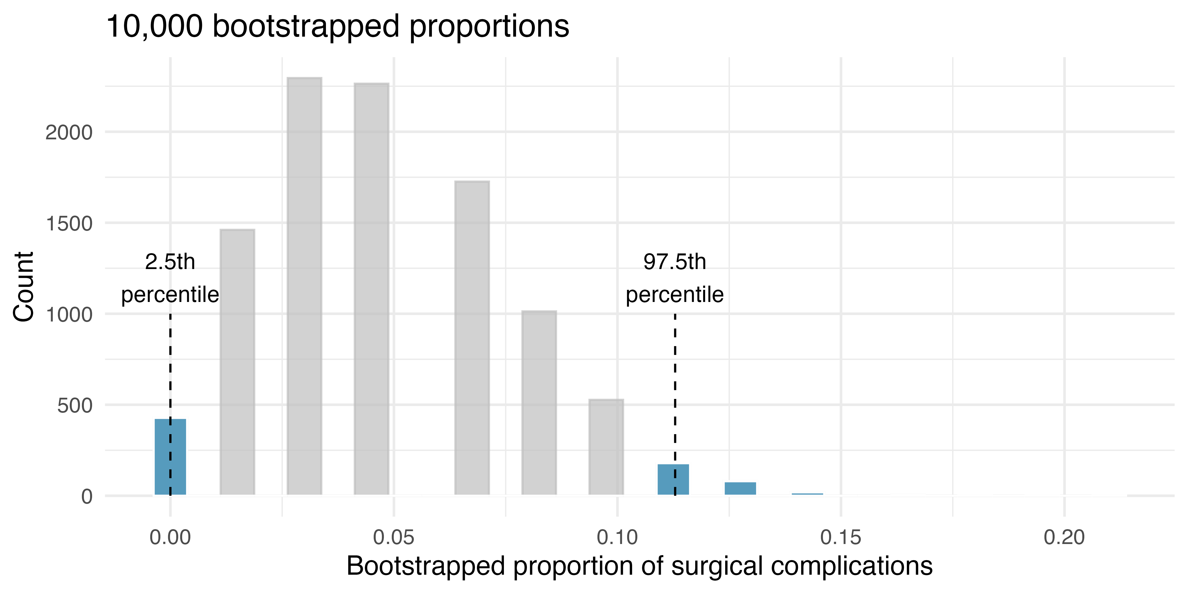
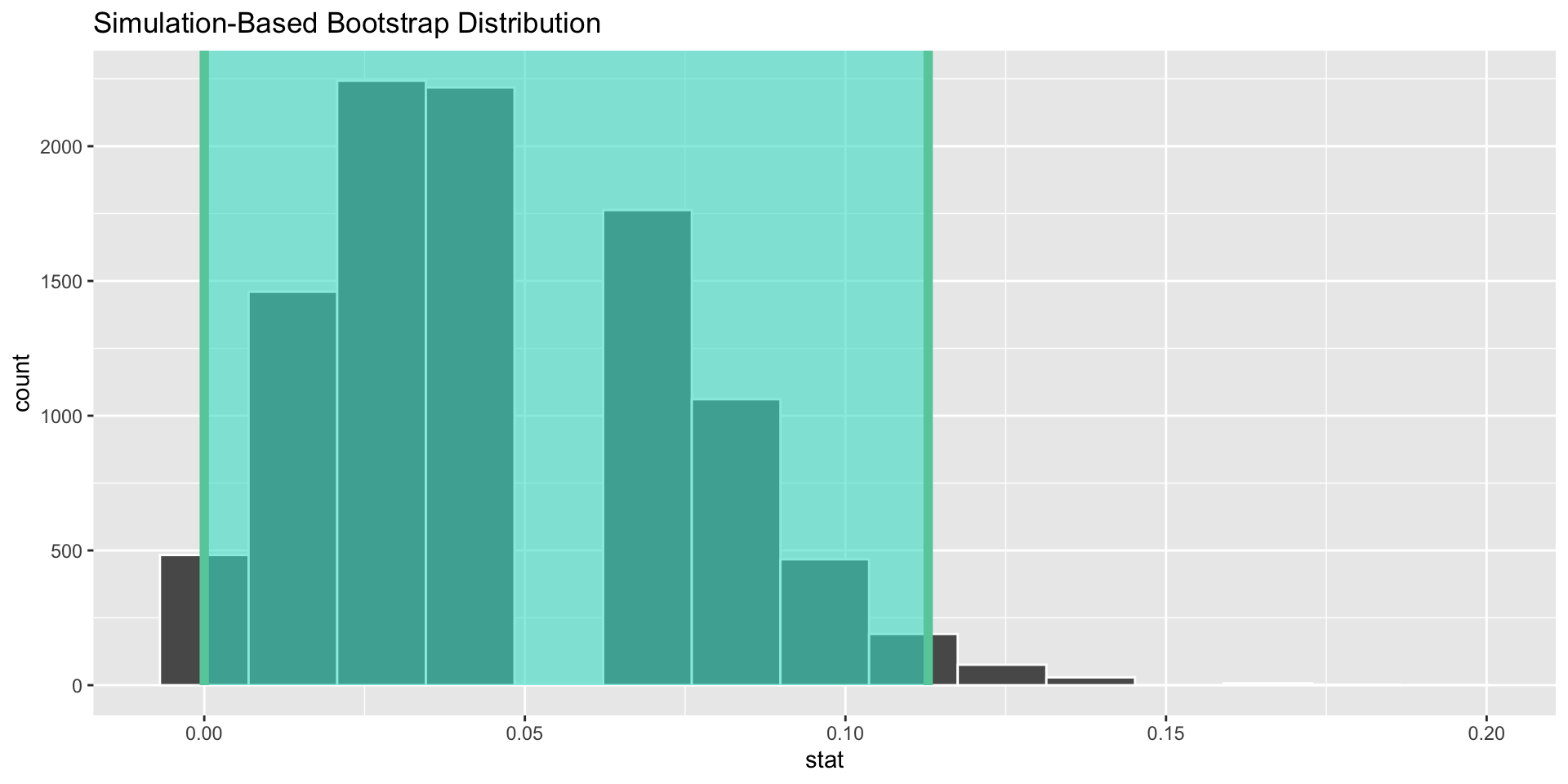
This is the distribution from 10,000 bootstrap simulations. They vary from 0 to 0.15. This variability leads us to believe that the true probability of complication (the underlying parameter \(p\)) is likely between 0 and 11.3% (the two dashed lines).
The Bootstrap Percentile Confidence Interval
That idea that we just discussed is called a bootstrap percentile confidence interval, or bootstrap interval for short.
We bootstrap on the context (in this case that means the nonparametric bootstrap: in this setting there is no null hypothesis, so no \(p_0\) to use to do a parametric bootstrap with).
If we want to be more certain that we capture the population parameter, i.e., increase our confidence level, should we use a wider interval or a smaller interval?
Width of an interval
If we want to be more certain that we capture the population parameter, i.e., increase our confidence level, should we use a wider interval or a smaller interval?
A wider interval.
Width of an interval
If we want to be more certain that we capture the population parameter, i.e., increase our confidence level, should we use a wider interval or a smaller interval?
A wider interval.
Can you see any drawbacks to using a wider interval?
Width of an interval
If we want to be more certain that we capture the population parameter, i.e., increase our confidence level, should we use a wider interval or a smaller interval?
A wider interval.
Can you see any drawbacks to using a wider interval?
If the interval is too wide it may not be very informative.1
Practice
Example 1 📊
Two scientists want to know if a certain drug is effective against high blood pressure. The first scientist wants to give the drug to 1000 people with high blood pressure and see how many of them experience lower blood pressure levels. The second scientist wants to give the drug to 500 people with high blood pressure, and not give the drug to another 500 people with high blood pressure, and see how many in both groups experience lower blood pressure levels. Which is the better way to test this drug?
All 1000 get the drug
500 get the drug, 500 don’t
Practice
Two scientists want to know if a certain drug is effective against high blood pressure. The first scientist wants to give the drug to 1000 people with high blood pressure and see how many of them experience lower blood pressure levels. The second scientist wants to give the drug to 500 people with high blood pressure, and not give the drug to another 500 people with high blood pressure, and see how many in both groups experience lower blood pressure levels. Which is the better way to test this drug?
All 1000 get the drug
500 get the drug, 500 don’t
Example 2: The GSS
The General Social Survey (GSS) collects information and keep a historical record of the concerns, experiences, attitudes, and practices of residents of the United States. Since 1972, the GSS has been monitoring societal change and studying the growing complexity of American society. Canada has been running a similar survey since 19851.
The GSS asks the question from the previous slide. Below is the distribution of responses from the 2010 survey:
All 1000 get the drug
99
500 get the drug, 500 don’t
571
Total
670
Parameter and Point Estimation
We would like to estimate the proportion of all Americans who have good intuition about experimental design, i.e., would answer “500 get the drug, 500 don’t”?
What are the parameter of interest and the point estimate?
Parameter and Point Estimation
We would like to estimate the proportion of all Americans who have good intuition about experimental design, i.e., would answer “500 get the drug, 500 don’t”?
What are the parameter of interest and the point estimate?
Parameter of Interest: Proportion of all Americans who have good intuition about experimental design
p: a population proportion
Point Estimate: proportion of sampled Americans who have good intuition about experimental design.
\(\hat{p}\): a sample proportion
Inference on a Proportion
What percent of all Americans have good intuition about experimental design, i.e., would answer “500 get the drug 500 don’t”?
We can answer this question using a confidence interval, computed with a bootstrap. We are given:
\(n = 670\)
\(x = 571\)
\(\hat{p} = 0.852\)
and told that the data are sampled randomly (so independent).
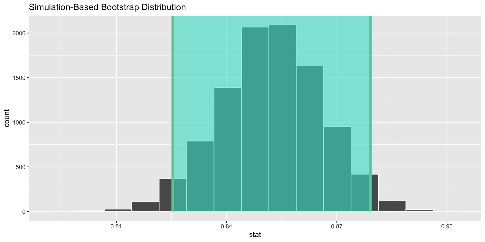
This range of values, \((0.825, 0.879)\) is a 95% bootstrap percentile confidence interval for the true underlying population proportion, \(p\), of Americans who have correct intuition about experimental design. Or, roughly, \((82.5, 87.9)\) %.
Plot
Can you see how 95% of the shaded area is in between the two green lines?
Exact Confidence Intervals for \(p\), using binom.test
We can also compute confidence intervals for \(p\) using the binom.test() function we mentioned recently. There’s on trick to it: unlike the case of hypothesis tests, all confidence intervals we compute in this class will be two-tailed. You have to set this correctly!
This means if you use binom.test() for both a hypothesis test and confidence interval in the same question, you might need to run it twice to get the right information!
The GSS Question: Hypothesis Test
test_result <-binom.test(x =571, n =670, p =0.5,alternative ="two.sided",conf.level =0.95)test_result
    Exact binomial test

data:  571 and 670
number of successes = 571, number of trials = 670, p-value < 2.2e-16
alternative hypothesis: true probability of success is not equal to 0.5
95 percent confidence interval:
 0.8230751 0.8782558
sample estimates:
probability of success
             0.8522388
The GSS Question: Confidence Interval
test_result$conf.int # this method is NOT compatible with dplyr
Thus a 95% exact binomial confidence interval for \(p\), the true underlying population proportion of Americans who have correct intuition about experimental design, is (0.823, 0.878).
Summary
So we have two different ways to access a confidence interval for \(p\):
Version 1: Use the binomial distribution, and binom.test().
Version 2: Use infer to create a bootstrap distribution, then extract
Readings
The contents of the latter part of this lecture come exclusively from Chapter 12 of Introduction to Modern Statistics (2e).