Lecture 12 - Single Proportion Hypothesis Testing
MATH 1051
Trent University
Hypothesis Testing Steps: Version 1
- Define the population parameter of interest and then state the null and alternative hypotheses (\(H_0\) and \(H_A\)) in reference to that parameter.
- Check assumption (independent random samples).
- Calculate test statistic from observations
- Find the \(p\)-value associated with the test statistic observed and the null distribution (using sum(dbinom()))
- Make a statistical decision (reject, or fail to reject, \(H_{0}\)).
- State a conclusion in the context of the question.
This was the method we did last week, and demonstrated on Friday.
Today
Today we are going to develop an alternative framework (Hypothesis Testing: Version 2) for testing hypotheses (single proportion) which does not use the binomial distribution. It is a fully non-parametric approach to answering the same question we’ve already done. That is:
Given the observed data and the test statistic, do we have evidence to support the extraordinary claim of the alternative hypothesis?
Philosophy
- Generally speaking, statistics is about the quantification of uncertainty.
- We want to be able to determine how uncertain our estimate (point estimate) of a quantity (population parameter) is, under some very mild assumptions.
- In a perfect world, what we would do in order to determine this is to repeat our experiment.
- In the medical consultant case from the previous lectures, we might take another sample of that consultant’s patients, of the same size (62), and see how many experienced complications.
- If we could do this an infinite number of times (or perhaps 14,000,605?) in a multiverse setting, we could see how variable the outcomes were, all under the same assumptions:
- the same consultant, the same practice, the same surgery, etc..
This leads us to a new idea: the bootstrap.
The Bootstrap
- The bootstrap is a statistical algorithm developed by Bradley Efron in 1978, with one key insight:
- we would like to sample from a population, but we don’t have access to it.
- What we do have is data.
- Can we somehow use the data to replace the need for the population?
And the answer is: yes!
Intuition
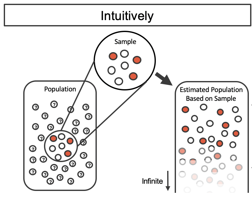
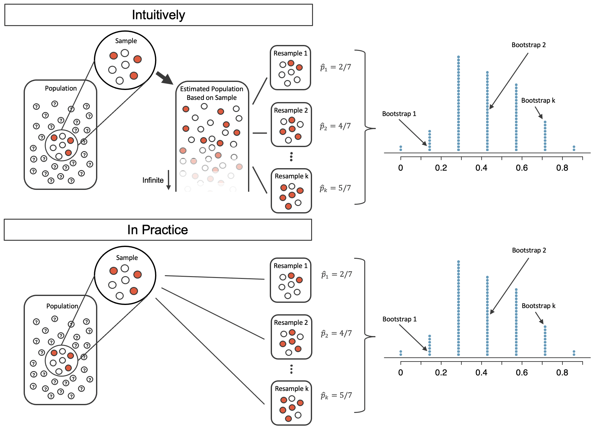
The sample in this case has 3 red and 4 white marbles, so the estimated population is 3/7 red and 4/7 white.
Intuition 2
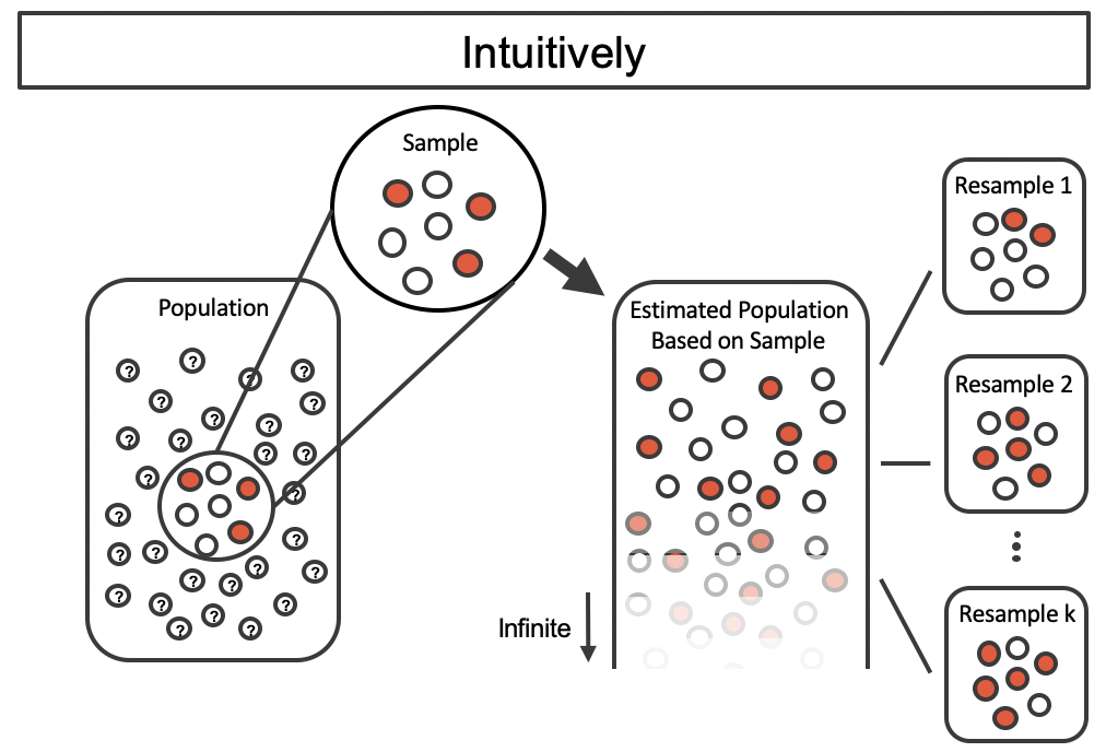
This “fake” (estimated) population can then be drawn from in order to see how variable samples would be if drawn from a 3/7 and 4/7 distribution population. This is a measure of sample variability.
Intuition 3
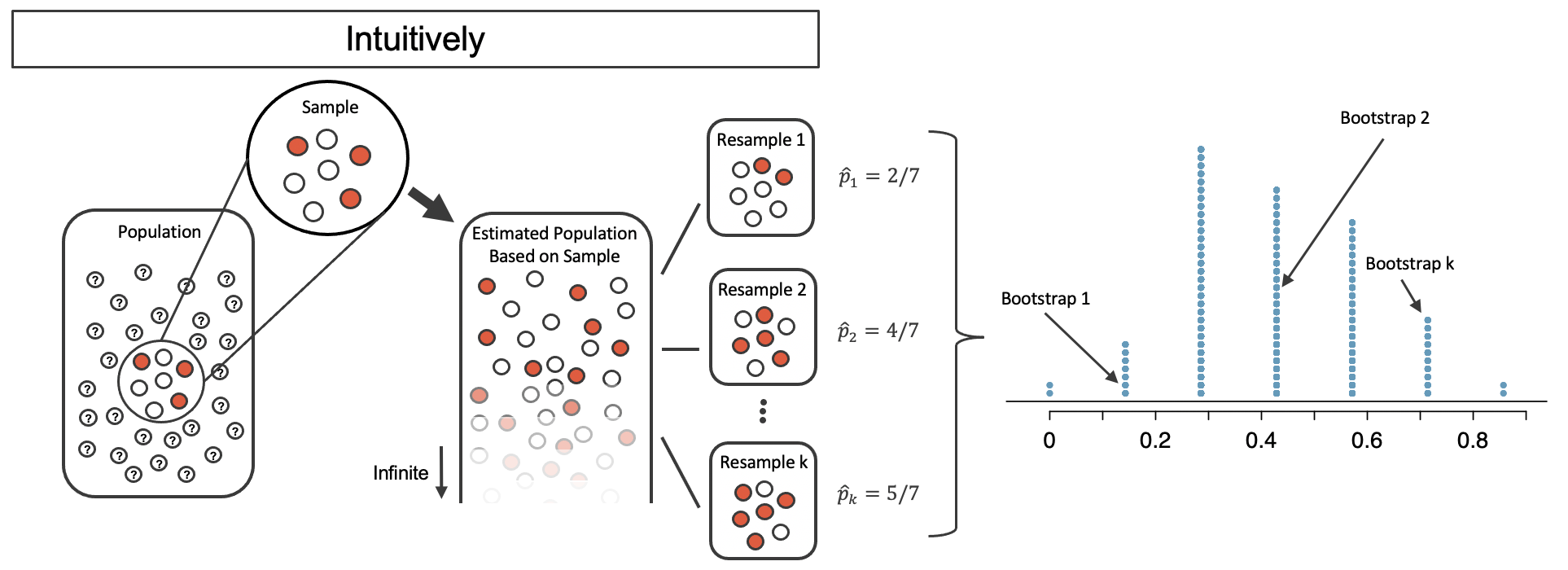
If we then summarize each of these resamples taken from the fake population by computing the proportion that are red, we get a distribution (and since it came from this bootstrap algorithm, we call it a bootstrap distribution) of \(\hat{p}\).
In Practice
Unfortunately, working with a theoretically infinite population is really hard for computers to manage. So we need a workaround. Instead of taking the sample, and then making the estimated population, instead we just sample with replacement from the original sample. This has exactly the same effect.
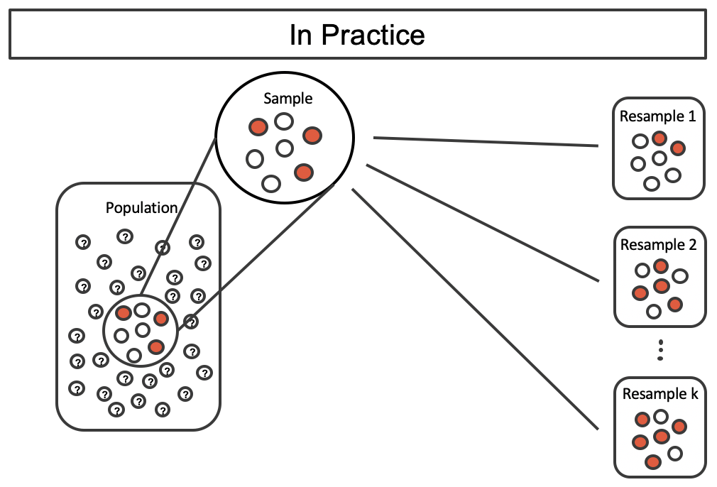
Overall Algorithm: Comparison
An Example: The Medical Consultant Again
If we apply the bootstrap sampling process to the medical consultant example, we consider each client to be one of the marbles in the bag.
There will be:
- 59 white marbles (no complication); and
- 3 red marbles (complication).
If we choose 62 marbles out of the bag (one at a time with replacement) and compute the proportion of simulated patients with complications, then this “bootstrap” proportion represents a single simulated proportion from the “resample from the sample” approach.
An Example: The Medical Consultant Again
Quick reminder: the consultant had 62 patients, 3 of whom had complications.
She stated that her complication rate (proportion of patients with complications) was better than the national average of 10%.
\[ H_{0}: p \geq 0.1 \quad \text{vs} \quad H_{A}: p < 0.1 \]
- \(p_{0} = 0.1\quad\) (null value)
- \(n = 62\quad\) (sample size)
- \(x = 3\quad\) (number of “successes”)
- \(\hat{p} = \frac{3}{62}\quad\) (sample proportion)
An Example: The Medical Consultant Again
If we apply the bootstrap sampling process to the medical consultant example, we consider each client to be one of the marbles in the bag.
There will be:
- 59 white marbles (no complication); and
- 3 red marbles (complication).
An Example: The Medical Consultant Again
- 59 white marbles (no complication); and
- 3 red marbles (complication).
Process:
- choose 62 marbles out of the bag (one at a time with replacement)
- compute the proportion of simulated patients with complications
- proportion of red marbles
This “bootstrap” proportion represents a single simulated proportion from the “resample from the sample” approach.
Q: In a simulation of 62 patients, about how many would we expect to have had a complication?
An Example: The Results
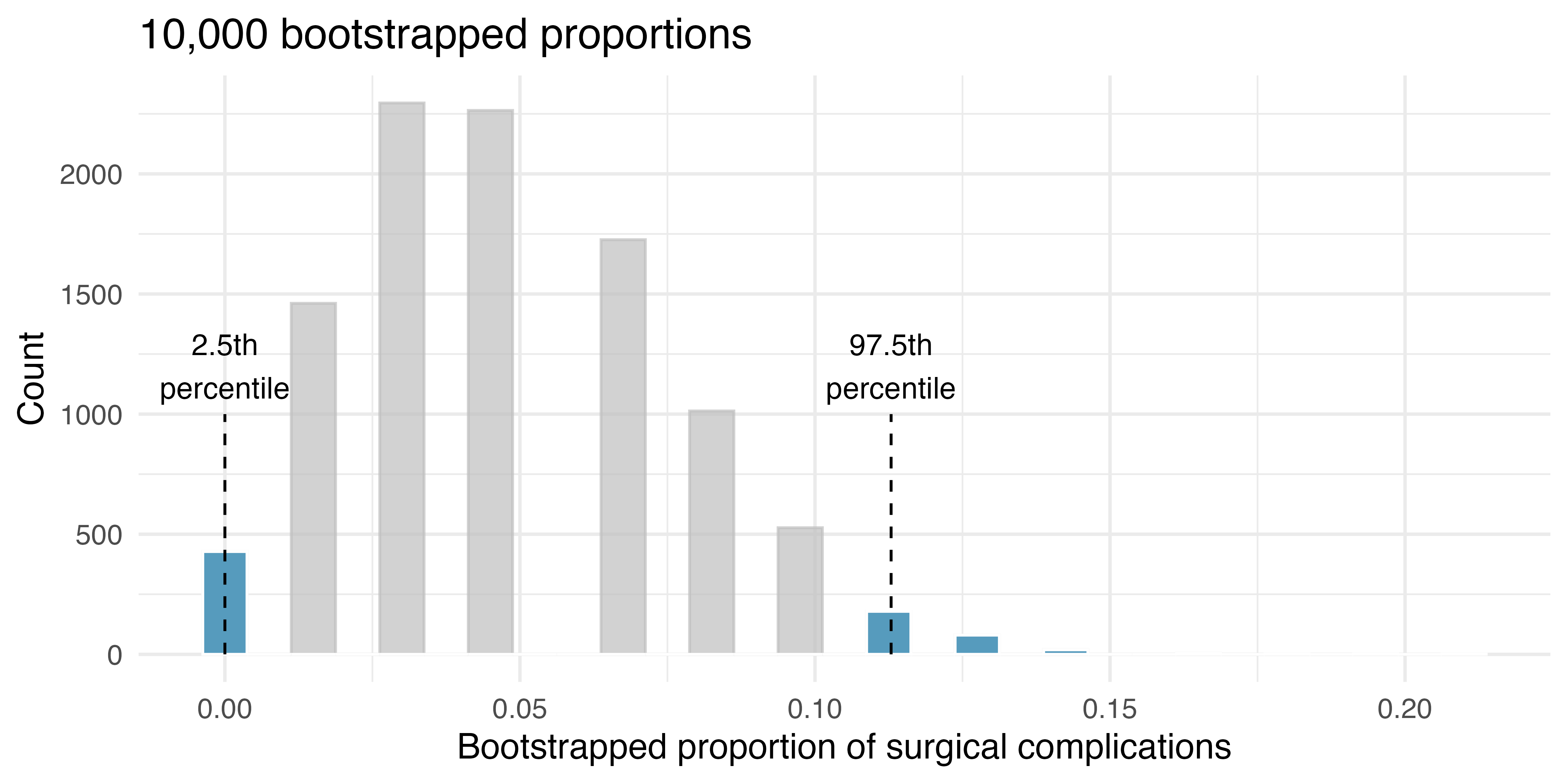
Figure: The original medical consultant data is bootstrapped 10,000 times. Each simulation creates a sample from the original data where the probability of a complication is \(\hat{p} = 3/62\).
However (this is really important!) this setup can’t quite let us answer a hypothesis test! We will return to this particular framework in a bit.
Bootstrap Hypothesis Tests
Using the Bootstrap to Conduct a Hypothesis Test
So how do we use this to answer a hypothesis test? It’s a very similar procedure to Version 1.
- Define the population parameter of interest and then state the null and alternative hypotheses (\(H_0\) and \(H_A\)) in reference to that parameter.
- Check assumption (independent random samples).
- Calculate the observed test statistic from the data.
- Find the \(p\)-value associated with the bootstrap distribution of the null: what proportion of the bootstrap replicates are as extreme as, or more extreme than, the observed test statistic.
- Make a statistical decision (reject, or fail to reject, \(H_{0}\)).
- State a conclusion in the context of the question.
“Of the Null”
In the last slide, we mentioned the “bootstrap distribution of the null”.
This is not the same as the bootstrap distribution of the statistic.
The bootstrap distribution used the sample proportion, \(\frac{3}{62}\) as the probability of observing a client with complications.
The bootstrap distribution of the null uses the null hypothesis value, \(p_0 = 0.10\)!
Be careful here.
The Results
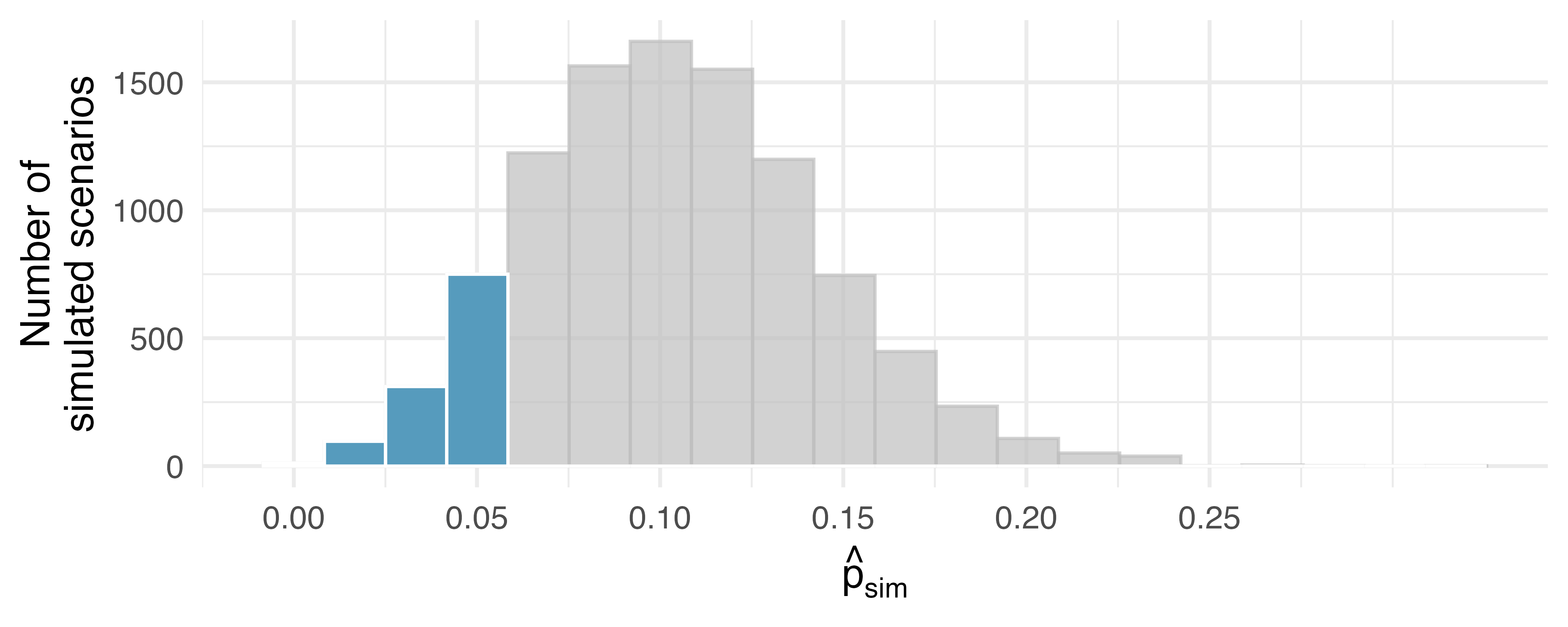
Note: this is not the same plot, or setup, as the previous plot. This is the parametric bootstrap (done based on the null of \(p_0 = 0.10\)); the previous was a nonparametric bootstrap (done based on \(\hat{p} = 3/62\)).
How This Works in Practice
- Under the null hypothesis, 10% of liver donors have complications during or after surgery.
- Suppose this rate was really no different for the consultant’s clients (for all the consultant’s clients, not just the 62 previously measured).
- If this was the case, we could simulate 62 clients to get a sample proportion for the complication rate from the null distribution.
- Simulating observations using a hypothesized null parameter value is often called a parametric bootstrap simulation; we can refer to it descriptively as “simulating under the null hypothesis claim.”
infer Approach for the Parametric Bootstrap
We discussed the existence of the infer package earlier. We implement the parametric bootstrap approach using the infer package.
Setup a data.frame with your observations:
and then set up the null:
Visualize
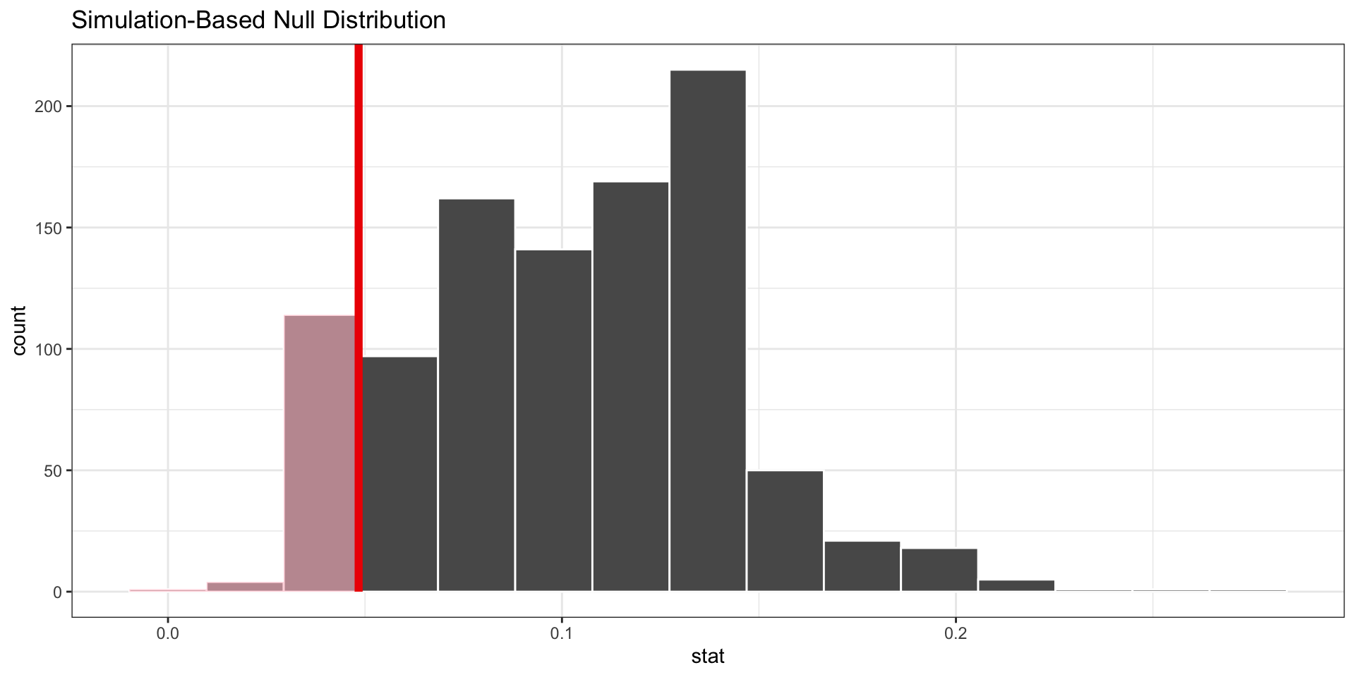
And the p-value
Compute:
# A tibble: 1 × 1
p_value
<dbl>
1 0.119So in the end, we have a number of ways of accessing the same thing. For the case of a single proportion, we can also just use binom.test() most of the time, but the infer package is really powerful, and allows us to do certain things that would otherwise be very tedious, so we will use both.
Summary
Version 1, Method 1
The method from earlier. Consider the null, assume independence and Bernoulli, so you have a binomial. Compute manually.
Version 1, Method 2
The method from earlier, but using a function to wrap it.
Exact binomial test
data: 3 and 62
number of successes = 3, number of trials = 62, p-value = 0.121
alternative hypothesis: true probability of success is less than 0.1
95 percent confidence interval:
0.0000000 0.1203362
sample estimates:
probability of success
0.0483871 [1] 0.1209787Version 2
The bootstrap approach, which simulates a population, then examines it. We can do this as a parametric bootstrap (the only way allowable for single proportions) using the infer package:
set.seed(12345)
null_dist <- surgery |>
  specify(response = Outcome, success = "Complication") |>
  hypothesize(null = "point", p = 0.10) |>
  generate(reps = 1000, type = "draw") |>
  calculate(stat = "prop")
p_hat <- surgery |>
observe(response = Outcome, success = "Complication", stat = "prop")
null_dist |>
  get_p_value(obs_stat = p_hat, direction = "less")
# A tibble: 1 × 1
p_value
<dbl>
1 0.122Examples
Ecology Example
An ecologist is studying a native prairie plant species. Under historical conditions, about 60% of seeds successfully germinate. After a habitat restoration project, the ecologist plants 2,000 seeds and wants to test whether the germination rate has increased from 60%. She observes 1,260 germinated plants in her seed planting.
- What is the point estimate for the true proportion of the seeds that will germinate?
- Can the ecologist statistically state that “The germination rate of this species is more than 60%?”
Ecology Example: Point Estimate
The point estimate is the proportion of seeds successfully germinated:
\[ \hat{p} = \frac{1260}{2000} \]
Ecology Example: Hypothesis Test
We start by stating the context. We have an ecologist, who planted 2,000 (\(n\)) seeds of a particular species. Of these 2,000 seeds, 1,260 (\(x\)) were successfully germinated after the restoration project. The ecologist wishes to write a paper and be able to confidently say that “More than 60%” of the seeds germinated after the restoration project.
The hypotheses for this setup are: \[ H_0: p \leq 0.6 \qquad \text{versus} \qquad H_A: p > 0.6 \]
And the point estimate is \(\hat{p} =\) 0.63. Let’s do the test, using the bootstrap method.
Ecology Example: Compute the p-value
# A tibble: 1 × 1
  p_value
    <dbl>
1  0.0028
Ecology Example: Conclusion
So we obtain a p-value of 0.0028, which means that we would estimate that if \(p = 0.6\), we would see a result as extreme as, or more extreme than, our observed point estimate / test statistic of 0.63 less than 1% of the time. This is a rare event, and seems implausible!
Therefore, we reject the null hypothesis, and conclude that the true underlying proportion of seeds that would germinate is indeed greater than 60% under the given conditions.
Another Example: DNA Profiles
Based on information from Canadian DNA Services, historic patterns suggest that around 80% of DNA samples collected using a particular protocol will yield a usable DNA profile for police services to reference. A particular forensic science agency that does sampling and analysis for the Toronto Police Service has been accused of performing erratic work, either outperforming the benchmark (doing better than expected) or underperforming the benchmark (doing worse than expected), depending on the time period and technicians working the cases. An external auditor reviews their cases from 2025 and finds that across 400 sampled crime scenes, 312 scenes yielded viable DNA profiles.
Use the sample data from this agency’s 2025 crime scenes to test the hypothesis put forward by the agency that they are performing at the expected level.
Another Example: Assumptions and Data
We are provided a null hypothesis (\(p = 0.80\)), and data (\(n=400\) and \(x = 312\)). Write the hypotheses:
\[ H_0: p = 0.80 \qquad \text{versus} \qquad H_A: p \neq 0.80 \]
In this case, “the claim” (by the agency!) gets put into the null hypothesis, because it is a claim about a specific value, not a claim about “being bigger than” or “being smaller than” or “not being equal to”. The accusation is in the alternative. Either is valid, and can be interpreted from the same solution path.
Another Example: Do the Test (Version 1)
    Exact binomial test

data:  312 and 400
number of successes = 312, number of trials = 400, p-value = 0.3174
alternative hypothesis: true probability of success is not equal to 0.8
95 percent confidence interval:
 0.7361567 0.8196440
sample estimates:
probability of success
                  0.78
This time we have to do \(2 \times\) because this is a two-tailed test, so we need both lower and upper cases. Since 312 is below the expected midpoint of the 400 cases (320), we would do \(\leq\) and then double it. Or just … read it from the binom.test output!
Another Example: Do the Test (Version 2)
set.seed(12345)
dna <- data.frame(Outcome = c( rep("Viable", 312),
                               rep("Not", 400 - 312))
                    )
p_hat <- dna |>
  observe(response = Outcome, success = "Viable", stat = "prop")

null_dist <- dna |>
  specify(response = Outcome, success = "Viable") |>
  hypothesize(null = "point", p = 0.80) |>
  generate(reps = 10000, type = "draw") |>
  calculate(stat = "prop")

p_val <- null_dist |>
  get_p_value(obs_stat = p_hat, direction = "two.sided")
p_val
# A tibble: 1 × 1
p_value
<dbl>
1 0.355A Note for Two Tails
NOTE: if you do this backwards, it gives a p-value \(> 1\). That’s ok, just flip it! But note that it’s impossible to be larger than 1!
In this case, since the parametric bootstrap p-value is 0.3548, we do not have evidence at the 5% level of significance to conclude that the proportion of cases handled by this agency produces anything other than the 80% viable samples suggested by the protocol. That is, we fail to reject the null, and cannot conclude that \(p \neq 0.80\).
Note: we never, ever conclude the null. In this case, that would be stating \(p = 0.80\). We do not know this!
Readings
The content of this lecture so far (the hypothesis tests for single proportions, many types) comes from Chapters 11, 12 and 16 in the Introduction to Modern Statistics (2e) textbook.