MATH 1051 - Lecture 11
Binomial Hypothesis Tests
Kat Clark & Wesley Burr
Trent University
Back to Probability
Returning to the Binomial
Recall the Binomial distribution that we learned about recently. This is the model used for repeated flips of a not-necessarily-fair coin. We write this as:
\[ X \sim \text{Binom}(n, p) \]
where \(n\) is the number of flips of the coin, and \(p\) is the probability of Heads. This may seem artificial, but it’s a really, really good model for success/fail events, which occur all the time in the sciences.
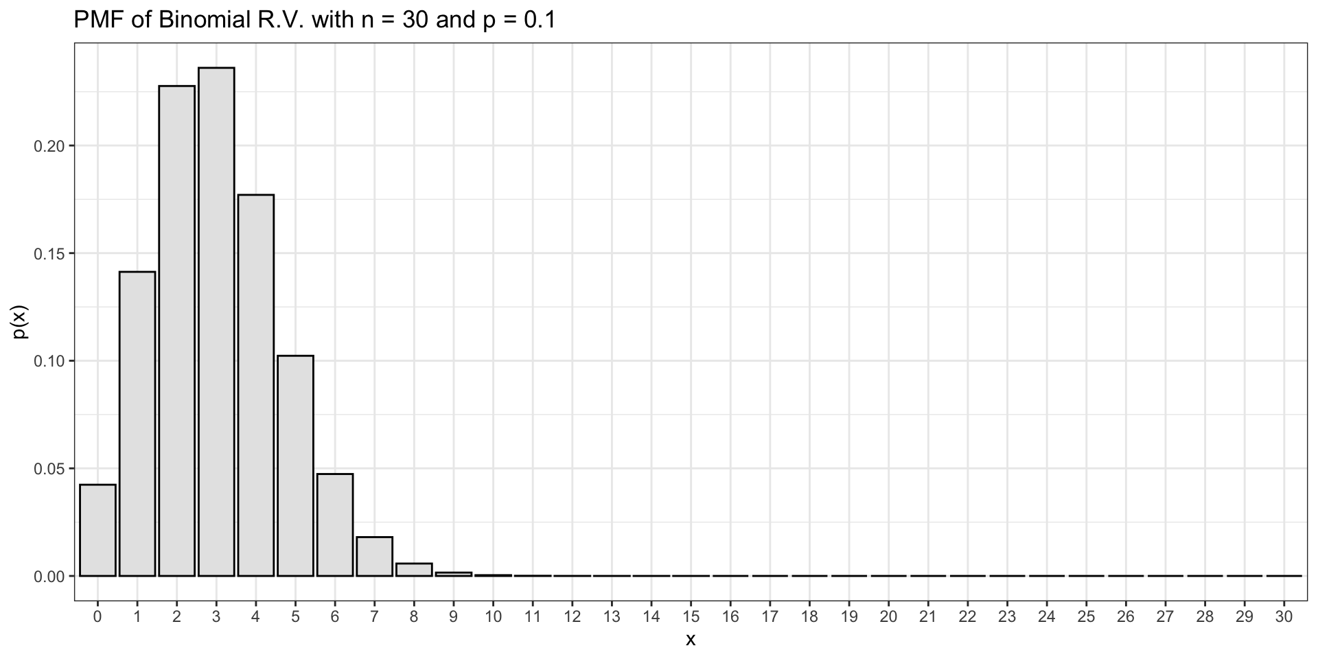
What Does a Binomial Distribution Look Like?
Let \(n=20\) and \(p=0.6\).
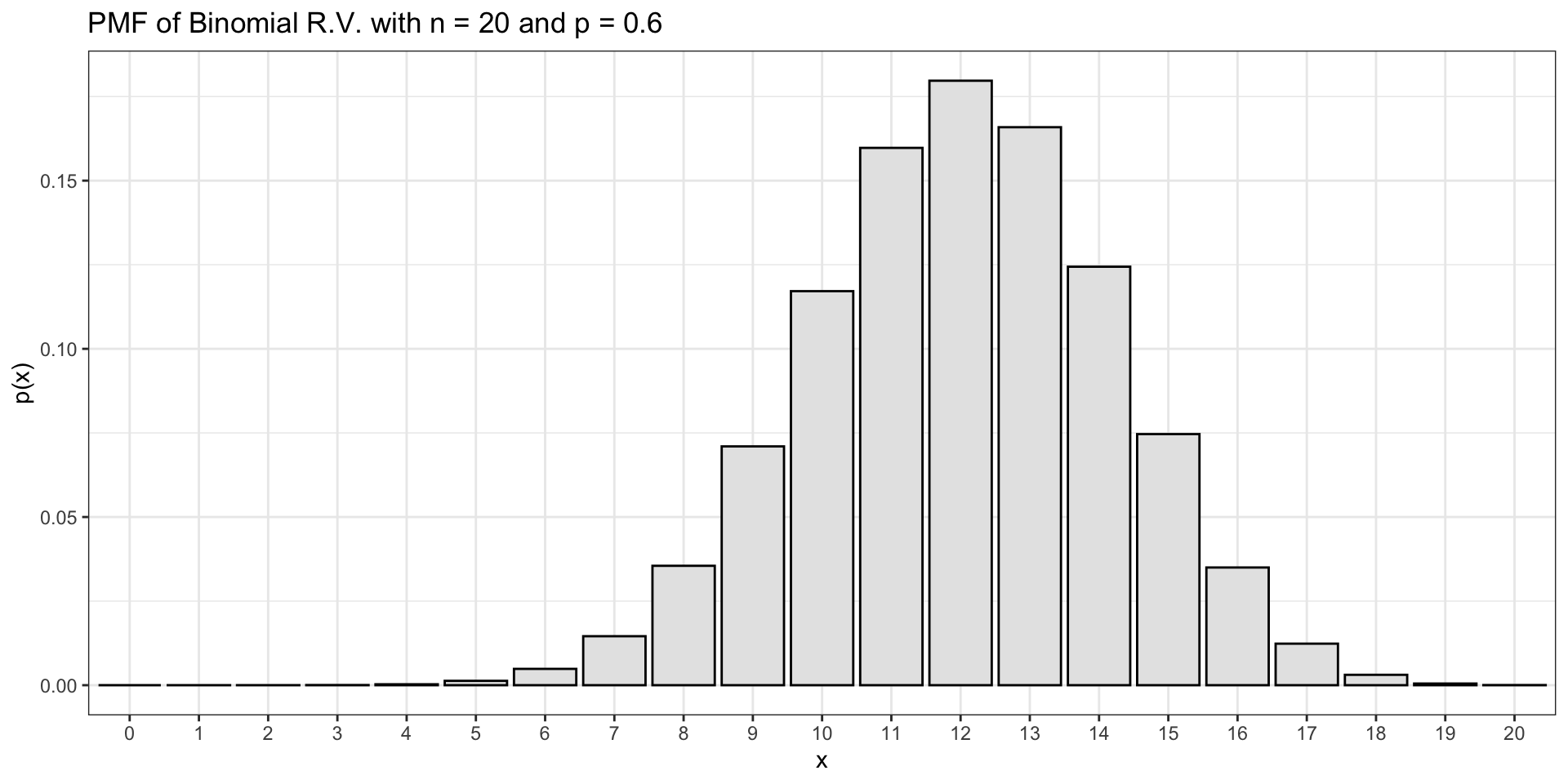
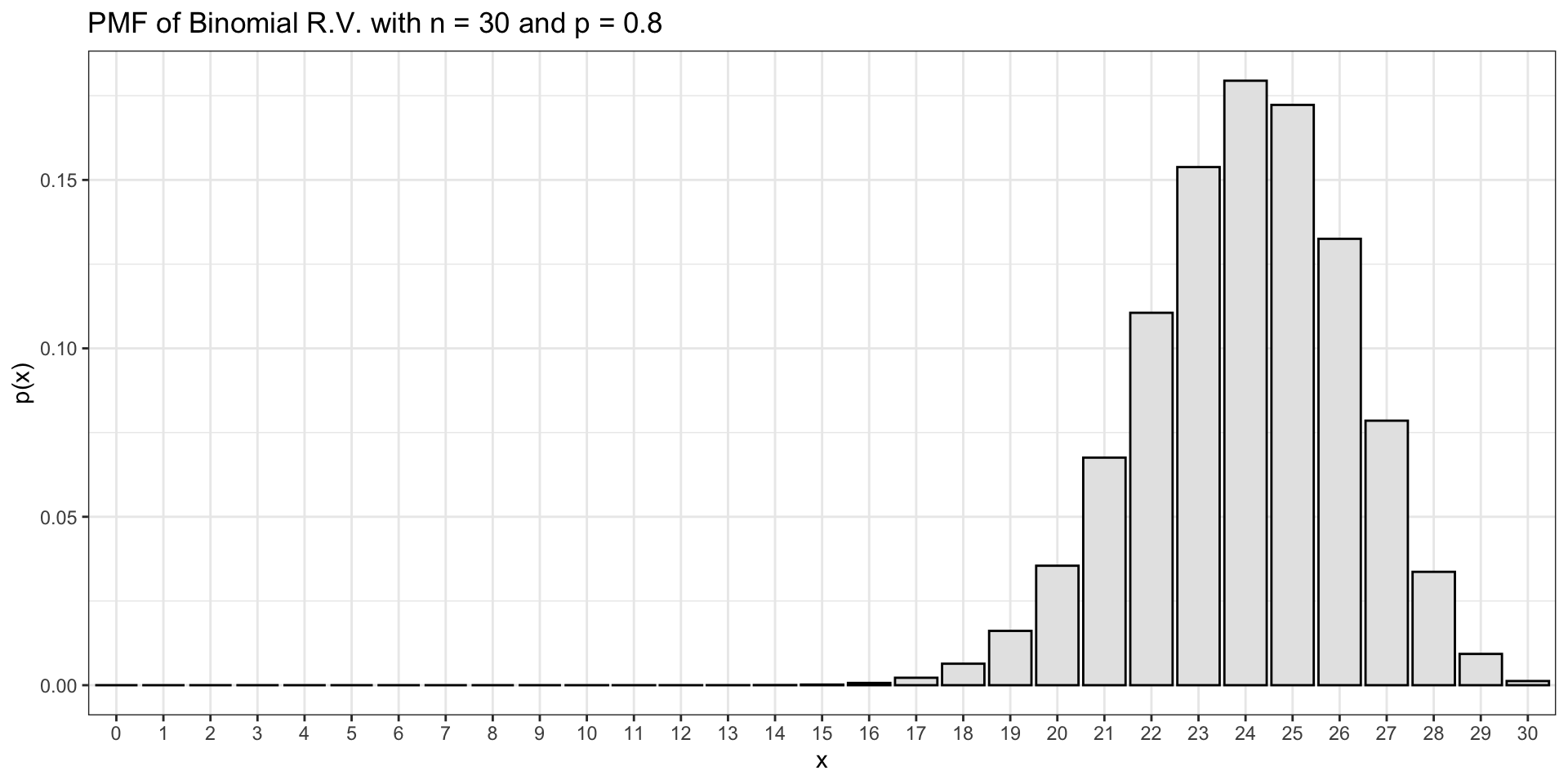
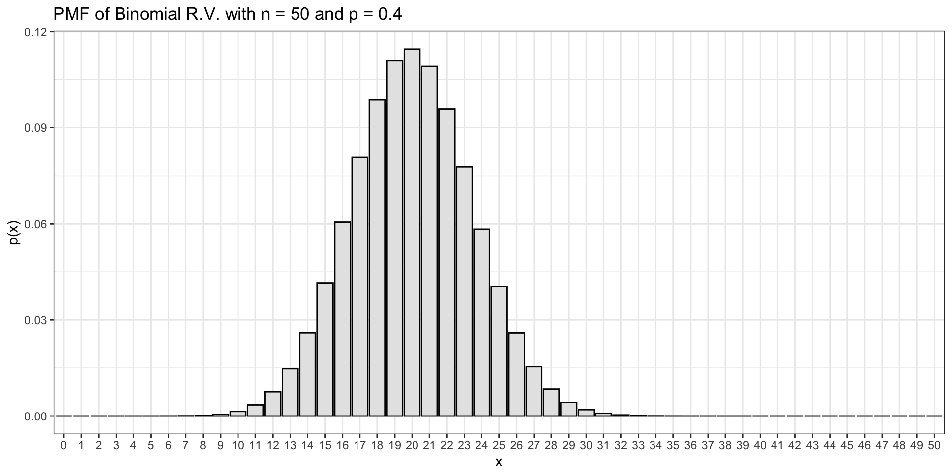
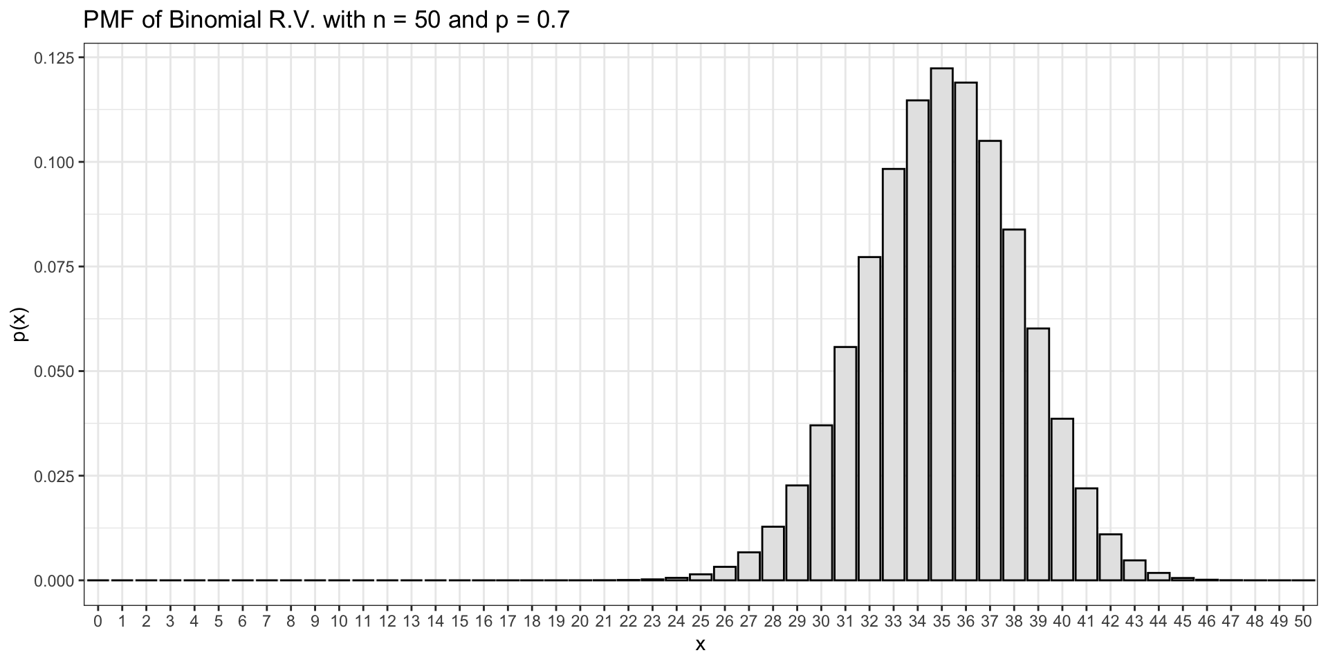
Some Other Examples
Measuring Probability
When dealing with the binomial distribution, we also want to answer probability problems, like we did with the normal recently. But unlike the normal, we don’t need to do integrals under a continuous curve: the binomial is discrete! That means we can just add stuff up.
           0            1            2            3            4            5
1.099512e-08 3.298535e-07 4.700412e-06 4.230371e-05 2.696862e-04 1.294494e-03
           6            7            8            9           10           11
4.854351e-03 1.456305e-02 3.549744e-02 7.099488e-02 1.171416e-01 1.597385e-01
          12           13           14           15           16           17
1.797058e-01 1.658823e-01 1.244117e-01 7.464702e-02 3.499079e-02 1.234969e-02
          18           19           20
3.087423e-03 4.874878e-04 3.656158e-05
This vector contains the probabilities of \(P(X=x)\) for \(x = 0\) through \(x = 20\). With these numbers, we can answer any probability question we want for this particular model.
Measuring Probability: \(P(X \leq 6)\)
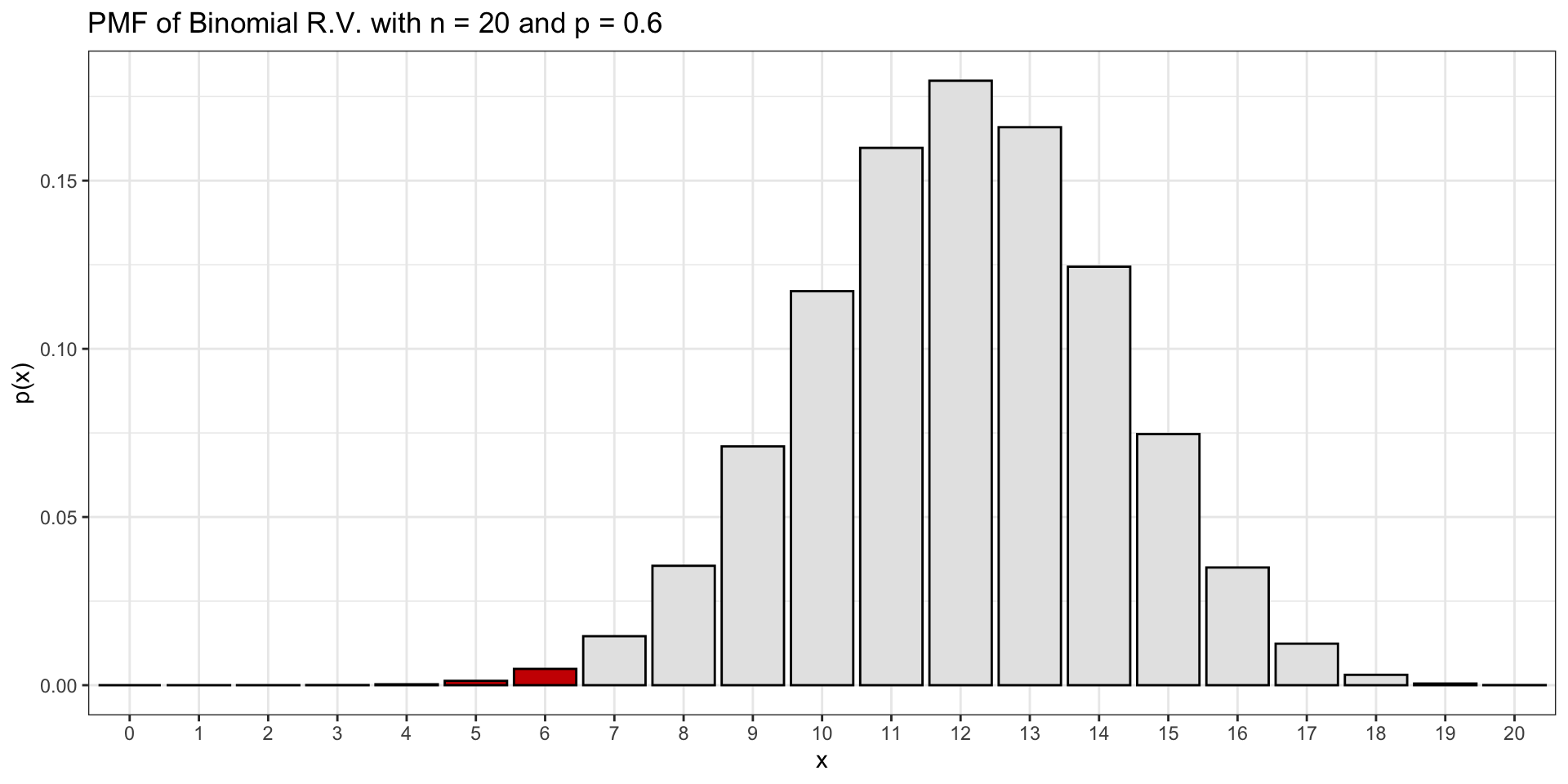
\(P(X \leq 6) =\) 0.0064659
Measuring Probability: \(P(X > 11)\)
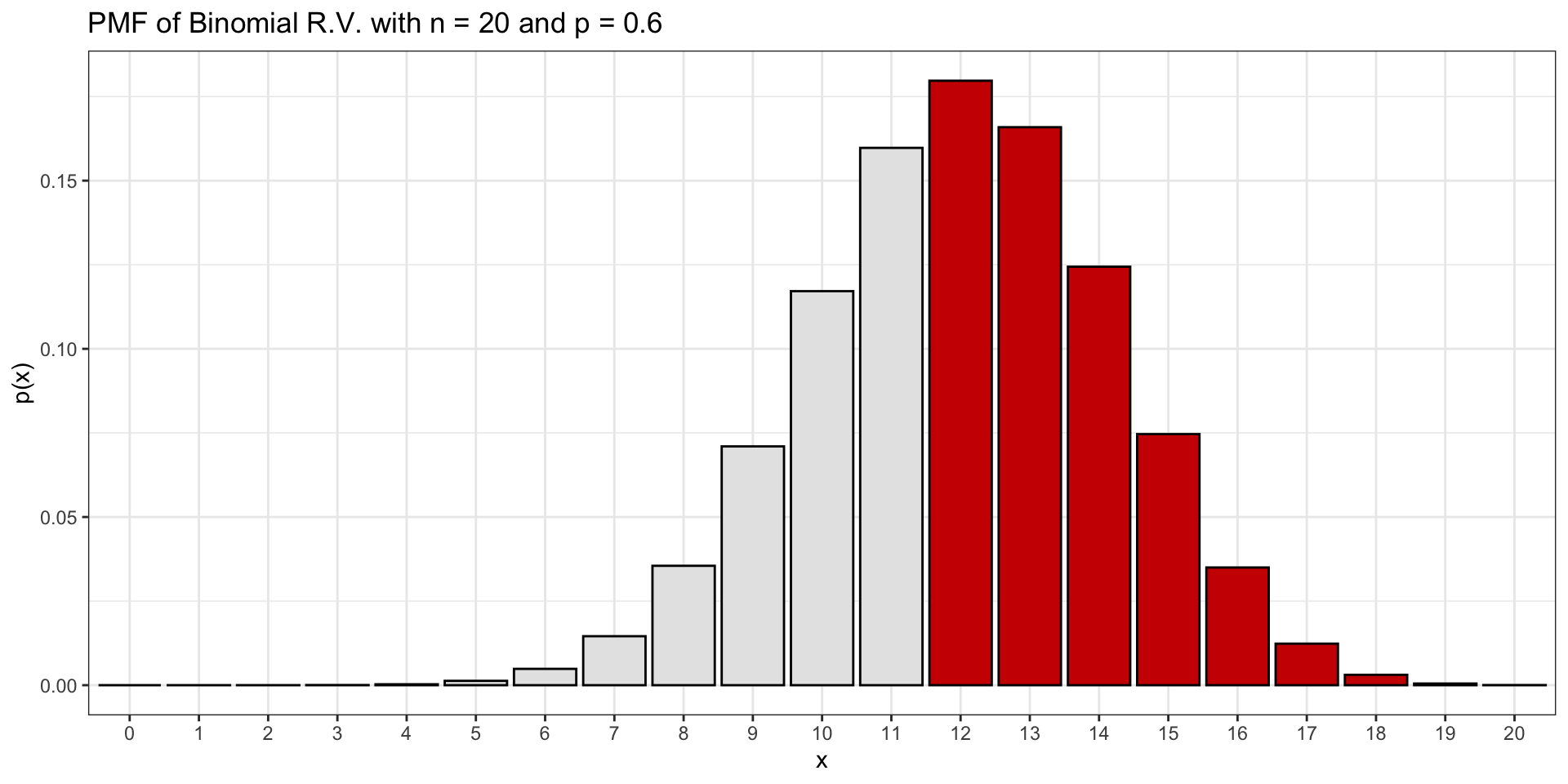
\(P(X > 11) =\) 0.5955987
Measuring Probability: \(P(7 < X \leq 13)\)
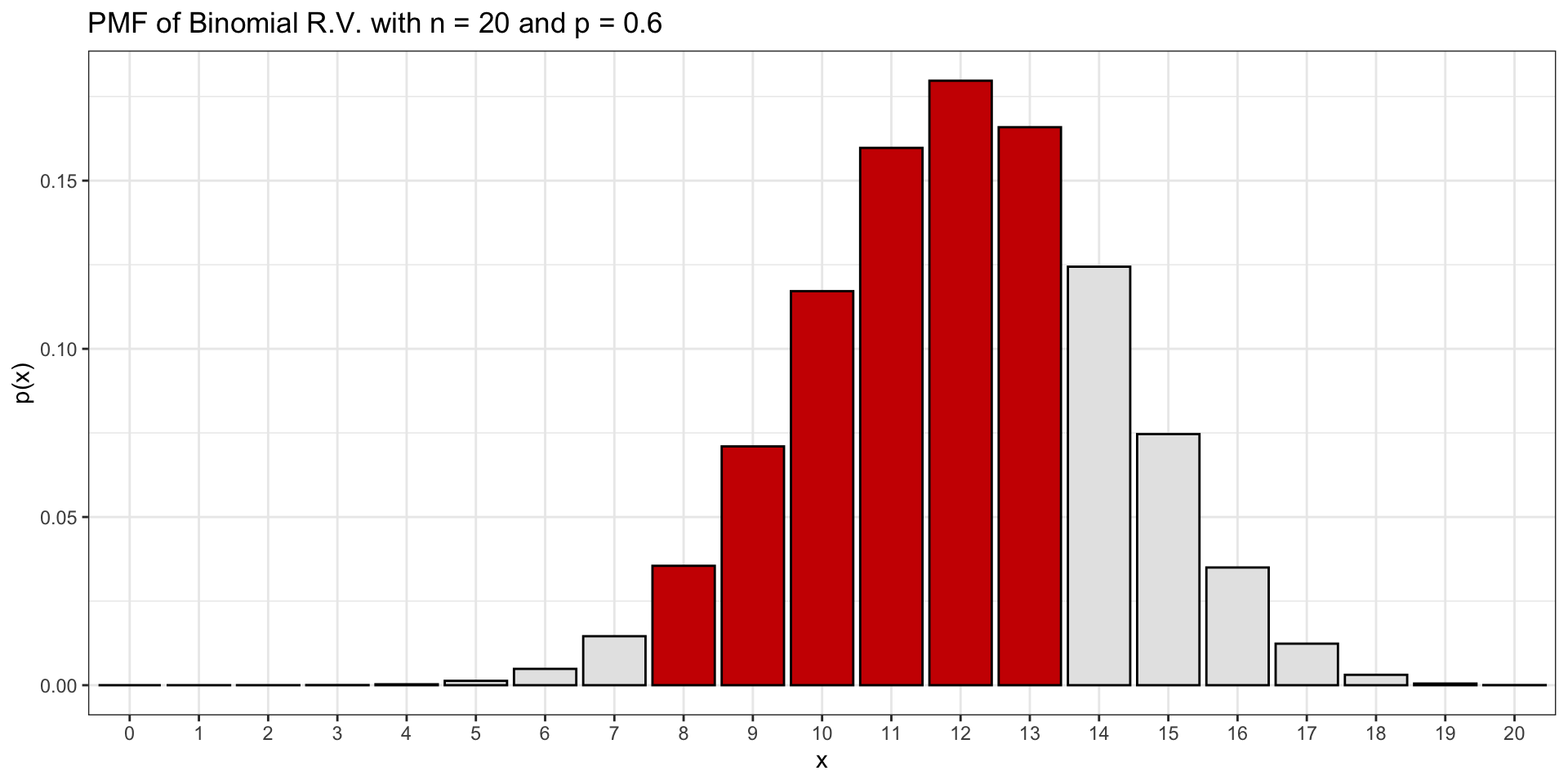
\(P(7 < X \leq 13) =\) 0.7289604
Discrete Simulation Results
- The binomial and “area under its curve” are not the same thing. But discrete simulation results and binomial distributions are very, very similar.
- They are both discrete objects (which means a finite, typically small, number of \(x\) possibilities).
- They both can be plotted as histograms. And we compute “area under the curve” in the same way: add up the rectangles!
Hypothesis Tests
Hypothesis Testing
- Last week, we handwaved an explanation of a hypothesis test.
- Let’s formally define the ideas, and set up the structure for one particular test, involving the binomials we just reviewed!
Hypothesis Test Definition
- A hypothesis test is a formal technique for evaluating two competing (mathematical statement) possibilities.
- In each scenario, we describe a null hypothesis which represents either a skeptical perspective or a perspective of no difference.
- We also have an alternative hypothesis, which represents a new perspective such as the possibility of a relationship between two variables or a treatment effect in an experiment.
- The alternative hypothesis is usually the reason the scientists set out to do the research in the first place, and is connected to the scientific hypothesis.
Null and alternative hypotheses.
The null hypothesis \((H_0)\) often represents either a skeptical perspective or a claim of “no difference” to be tested.
The alternative hypothesis (\(H_A\)) represents an alternative claim under consideration and is (for us, always!) represented by a range of possible values for the value of interest.
Setting Up \(H_{0}\) and \(H_{A}\)
When the hypotheses can be represented as a mathematical expression, the expression that contains equality is the null!
“Containing equality” means: \(=\), \(\leq\), or \(\geq\)
The Famous p-value
- The p-value is one of the most misunderstood concepts in all of science.
- Formally, it is: the probability of observing data at least as favourable to the alternative hypothesis as our current dataset, if the null hypothesis were true.
- We’ll often refer to this as the probability of seeing a result as extreme as, or more extreme than the observed statistic, under the assumption that the null is true.
Recall the simulation (10,000 replicates) we did for the gender bias study. We found results that were \(\geq\) the observed statistic (called the test statistic).
Those were results that were as extreme as (the \(=\)) or more extreme than (the \(>\)) the observed difference in proportions.
Is a Simulation the “Real” p-value?
- Technically speaking, when we run a simulation, regardless of how many replicates we use, we aren’t getting the “real” p-value.
- Think again about the gender bias study.
- We had 48 samples, 35 ‘successes’ and 13 ‘failures’.
- How many ways are there to choose 24 samples from this set of 48?
- That is … a really big number: 3,224,763,683,100.
- We’d need to observe over 3 trillion unique permutations of the data in order to get the exact p-value under the null.
- However, what we’ve discovered is that mathematically, doing “enough” simulations gets us really close.
Let’s try increasing numbers of simulations and see what happens for this case.
Results: Increasing Replicates
Making Decisions
- A hypothesis test is about making a decision.
- Given the data, how probable is the alternative hypothesis?
- Do we believe it is plausible and the actual truth of the situation?
- When the p-value is small, we say the results are statistically discernible (or often referred to as statistically significant).
- “small” is determined by us, the researchers before we run the test!
- This means the data provide such strong evidence against \(H_0\) that we reject the null hypothesis in favour of the alternative hypothesis.
Statistical Discernability
- The threshold is called the discernibility level (or significance level) and often represented by \(\alpha\).
- The value of \(\alpha\) represents how rare an event needs to be in order for the null hypothesis to be rejected.
- Historically, many fields have set \(\alpha = 0.05\) if the null hypothesis is to be rejected, but this varies widely.
- We say that the data provide statistically discernible (or statistically significant) evidence against the null hypothesis if the p-value is less than some predetermined threshold (e.g., 0.01, 0.05, 0.1).
A Little Bit of Language
Parameters
- In statistics, parameters are underlying properties, or characteristics, of populations.
- Consider “Canada”: If we restrict our attention to the population of Canada at 1149am on September 15th, 2024, and consider only citizens, permanent residents, and those possessing valid visas, who are currently physically present in Canada, at that moment in time, we have a fairly well defined population.
- There are approximately 40 million such people in Canada.
- Then, this population has a number of attributes.
- For example, average age.
- If we could take such a snapshot, we could measure the age of every member of that population, then take the average of those ages.
- We could similarly examine the average height, proportion with a defined disability, or even most common hair colour.
- For example, average age.
Parameters
- These attributes of populations are called parameters, and are usually restricted to considering only those that are numerical quantities (e.g., average weight, age, height, income, etc.).
- Most parameters are denoted by Greek letters, especially \(\mu\) (mean) and \(\sigma\) (standard deviation).
Parameters as Numeric Quantities
This doesn’t mean that the variable we are considering is numeric, simply that we are considering a numeric value.
E.g., Proportion of blue cars.
E.g., Count of people with an area code of 613.
Point Estimates
- When we gather data, we can compute the same functions as are used in the calculation of parameters.
- If the parameter is average age of Canadians, then the function is the average, so we can apply this same mathematical function to a data set.
- Instead of using Canada, let’s use all students who are present and accounted for at today’s class.
- There’s approximately 500 such students across the three sections.
- We can measure attributes from all of you, and then take the average.
- This is called a sample average because it’s computed on a sample of data.
- Additionally, this is a statistic.
- Statistics are often referred to as point estimates: they are a point, and they are used to estimate a parameter.
- The class’ average height can be used as an estimate (a statistical guess) for the average height of a larger population.
Connections to Hypothesis Tests
- Hypothesis tests are always about parameters.
- Hypothesis tests are computed using the data, which means using the statistic of interest, applied to the data.
- Thus, hypothesis tests let us take our point estimates, and determine whether the evidence supports some categorization of the underlying parameter.
Inference for Single Proportions
Single Proportion Tests
- We often encounter situations where we have gathered data (e.g., from a survey) where the responses can be categorized as: positive or negative; true or false; yes or no.
- A reasonable way to represent such data is via a proportion: the ratio of the number of “yes” results to the total number of trials.
- For example, we might have reproductive fitness in an ecological example, where we sample from 36 sites known to have been used by shorebirds to nest in the past.
- Of those 36 sites, 11 are observed to have active nesting occurring.
- Thus, the proportion of sites actively being used is 11/36, or 0.306.
Setting Up the Test: Version 1
- When doing a test (any test!), the first question we ask is: what is our parameter of interest and what statistic will be use to find a point estimate?
- That is, what population did we sample from, what have we observed, and what kind of statistic do we need to use?
- In single proportions, the parameter of interest is the population proportion and the point estimate is the sample proportion: just the ratio of successes to trials (number of observed “successes” divided by the number of observations).
- We denote this as \(\hat{p}\).
- It is our best guess for the truth, \(p\) (the population proportion).
- We’ll talk more about this in the coming weeks.
- We take the parameter, and set up a hypothesis around it.
- This comes with three things: (1) the null hypothesis; (2) the alternative hypothesis; (3) any assumptions that we had to make to make this work.
Setting Up the Test: Version 1 - The Null
In the case of the parameter of interest being the population proportion, our null hypothesis will written with respect to \(p\).
This is some underlying truth about the population that we don’t know.
So our null will always be a statement like:
\[ H_0: p = ??? \]
Later, we will use the sample proportion, \(\hat{p}\), to make a statistical decision.
Setting Up the Test: Version 1 - The Alternative
- As with the null, we are talking about the population proportion of some attribute, \(p\).
- There are three options for an alternative hypothesis.
- We can think that: \(p > ??\) OR \(p < ??\) OR \(p \neq ??\)
- That’s it.
- We can think that: \(p > ??\) OR \(p < ??\) OR \(p \neq ??\)
- The alternative is that \(p\) is greater than something, less than something, or not-equal-to something.
And what is that something \(??\)? Always the value in the null hypothesis!
Note
Think about what this “test” is: it is a binary decision. Either you decide the evidence (from the data) isn’t rare and odd, so you can’t reject the null; or you decide the evidence is rare, and odd, so you reject the null.
In the latter case, you don’t actually know what the truth is, just that it isn’t the null. So \(>\), \(<\) or \(\neq\) is the best you can do.
Setting Up the Test: Version 1 - The Assumptions
- What assumptions are necessary to make this work?
- Not a lot!
- We have to assume that the samples are independent random samples taken from a population, and then that the proportion is computed in a sensible way.
- These are essentially always true.
- Then, because of the key assumption (independence), we get something really powerful: independent samples (trials) taken from a population and a count of “successes”.
- We take this count and divide by the total number of observations which results in a proportion, distributed as a Binomial random variable.
In such a case, we say that the null distribution is a Binomial.
Organ Donation Example
- People providing an organ for donation sometimes seek the help of a special “medical consultant”.
- These consultants assist the patient in all aspects of the surgery, with the goal of reducing the possibility of complications during the medical procedure and recovery.
- Patients might choose a consultant based in part on the historical complication rate of the consultant’s clients.
- One consultant tried to attract patients by noting the average complication rate for liver donor surgeries in the US is about 10%, but her clients have only had 3 complications in the 62 liver donor surgeries she has facilitated.
- She claims this is strong evidence that her work meaningfully contributes to reducing complications (and therefore she should be hired!).
Perform a test where you require that the observed outcome be very rare (less than 0.02 probability) in order to believe the exceptional claim she is making.
Example: Key Information
- average complication rate: 10%
- her patients: 3 in 62
- claims this is strong evidence that she is better than average
Convert this into math. From the provided population average:
\[ H_0: p = 0.10 \]
Her exceptional claim: that she is better than the average, and her patients experience less complications than average.
\[ H_A: p < 0.10 \]
Finally, from the patient information:
\[ X = 3 \quad \text{ or } \quad \hat{p} = 3/62 = 0.0483871 \]
We don’t round!
Example: Doing the Test
- We can assume that each patient is independent of the other patients, so we have 62 randomly sampled observations from a larger population of “people who undergo liver transplants as donors”.
- The number of complications in our sample follows a Binomial distribution with \(n=62\).
- The probability of a complication is the population average, \(p=0.10\).
That is:
\[ X \sim \text{Binomial}(n=62, p=0.10) \]
- In our sample, we observed \(X=3\) complications.
- Doing the “test” is really just answering the following question:
- If complications truly occur 10% of the time (that is, under the null hypothesis), what is the probability of observing 3 complications or fewer in a sample of 62 patients?
Example: A Pictorial Representation
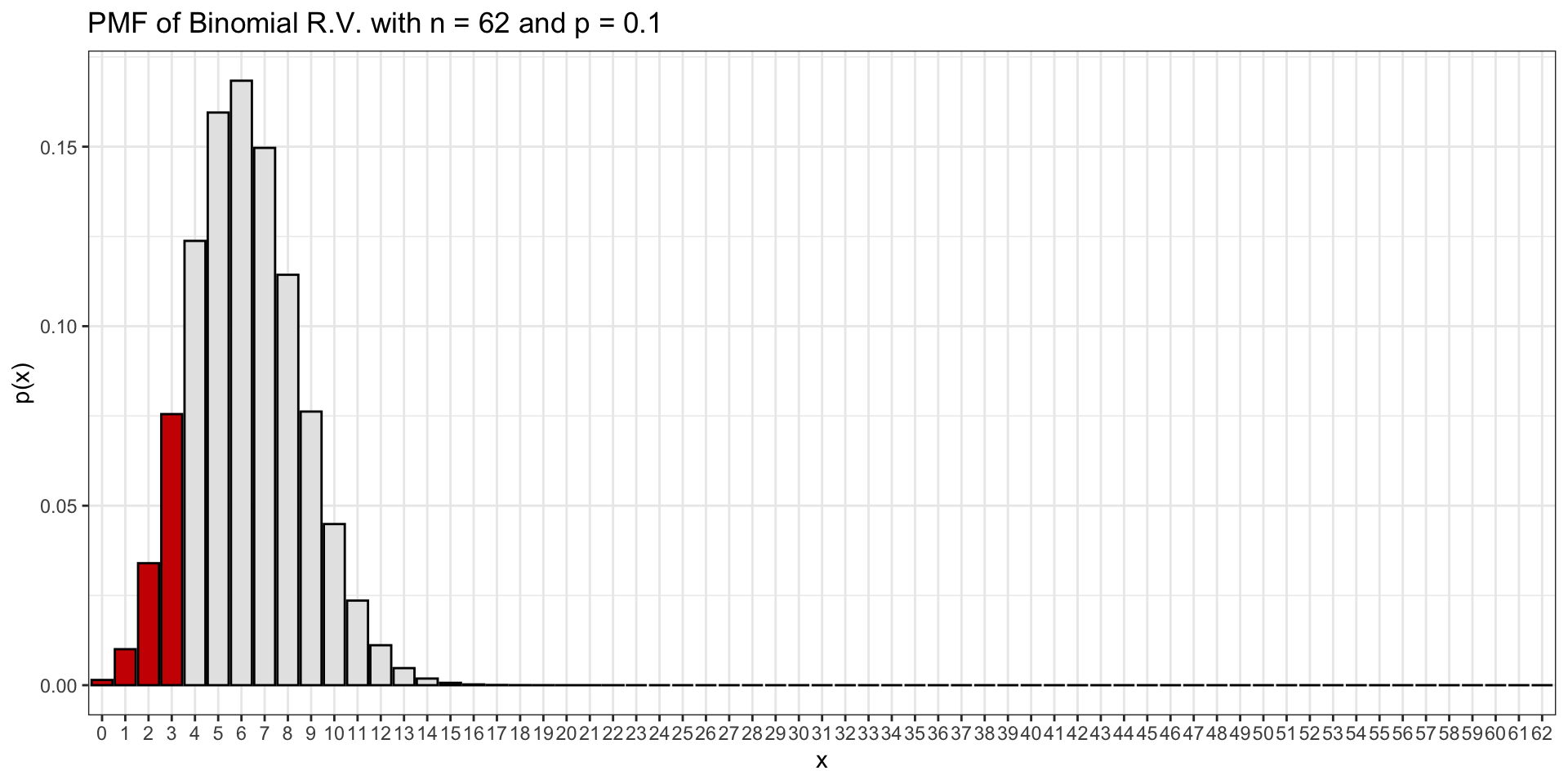
Example: Formally computing the p-value
- Under the null, \(\hat{p}\) is a Binomial with \(n=62\) and \(p = 0.10\).
- In that case, we would expect to see a result “As extreme as, or more extreme than” (in the direction left) 3-in-62 with probability 0.1209787. Or around 12% of the time.
- Is this rare?
- 12% is not that low.
- We’d expect to see that fairly often, just by chance: 12% of the time!
- Thus, the consultant’s “evidence” is not very strong, and we see no convincing reason to conclude that she is better than average at helping her patients with their transplant donations.
- In formal statistical language, we “fail to reject the null hypothesis” and “conclude that there is insufficient statistical evidence to think that \(p < 0.10\) for this consultant”.
Recap
- We’ve spent a lot of time today developing the general framework for hypothesis testing.
- We considered how to design and test an example with one proportion.
- We will continue this development in the coming lectures.
- After a short break, we’ll solve some hypothesis tests together.
Readings for Today
Today’s topic was drawn from Chapter 16 of Introduction to Modern Statistics (2e).