MATH 1051 - Lecture 10

Introduction to Statistical Inference

Kat Clark & Wesley Burr

Trent University

Volunteer Notetakers Needed

Help a Classmate. Build Your Resume.

Share the notes you’re already taking
Support students registered with Accessibility Services
Eligible for your Co-Curricular Record
Reference letter or certificate available upon request

🔗 trentu.ca/wellness/cat/notetaking
📧 notetaking@trentu.ca

Sign up through the SAS Portal

Case Study: Gender Discrimination

Gender Discrimination

In 1972, as a part of a study¹ on gender discrimination, 48 male bank supervisors were each given the same personnel file and asked to judge whether the person should be promoted to a branch manager job that was described as “routine”.
The files were identical except that half of the supervisors had files showing the person was male while the other half had files showing the person was female.
It was randomly determined which supervisors got “male” applications and which got “female” applications.
Of the 48 files reviewed, 35 were promoted.
The study is testing whether females are unfairly discriminated against.
Is this an observational study or an experiment?

Data

At a first glance, does there appear to be a relationship between promotion and gender?

	Promoted
	Yes	No	Total
Gender
Male	21	3	24
Female	14	10	24
Total
	35	13	48

% of males promoted: 21 / 24 * 100 = 87.5

% of females promoted: 14 / 24 * 100 = 58.3

% difference: 87.5-58.3 = 29.2

Practice

We saw a difference of almost 30% (29.2% to be exact) between the proportion of male and female files that are promoted. Based on this information, which of the below is true?

If we were to repeat the experiment we will definitely see that more female files get promoted. This was a fluke.
Promotion is dependent on gender, males are more likely to be promoted, and hence there is gender discrimination against women in promotion decisions.
The difference in the proportions of promoted male and female files is due to chance, this is not evidence of gender discrimination against women in promotion decisions.
Women are less qualified than men, and this is why fewer females get promoted.

Practice

We saw a difference of almost 30% (29.2% to be exact) between the proportion of male and female files that are promoted. Based on this information, which of the below is true?

If we were to repeat the experiment we will definitely see that more female files get promoted. This was a fluke.
Promotion is dependent on gender, males are more likely to be promoted, and hence there is gender discrimination against women in promotion decisions. Maybe!
The difference in the proportions of promoted male and female files is due to chance, this is not evidence of gender discrimination against women in promotion decisions. Maybe!
Women are less qualified than men, and this is why fewer females get promoted.

Two Competing Claims

“There is nothing going on.” (Null Hypothesis)

Promotion and gender are independent.

No gender discrimination.

Observed difference in proportions is simply due to chance.

versus

“There is something going on.” (Alternative Hypothesis)

Promotion and gender are dependent.

There is gender discrimination.

Observed difference in proportions is not due to chance.

Hypothesis Testing

The secret ingredients

Setup your hypotheses (\(H_{0}\) and \(H_{A}\)).
Test assumptions (e.g. normality, independence, etc.)
Calculate your test statistic under \(H_{0}\)
Find the \(p\)-value associated with Step 3
Determine whether to reject or not reject the null hypothesis:
- compare your p-value to a significance level
Conclusion: There is …
- evidence to support rejecting the null hypothesis (reject \(H_{0}\))
  OR
- not enough evidence to support rejecting the null hypothesis (fail to reject \(H_{0}\))

Hypothesis Tests as a Trial

Hypothesis testing is very much like a court trial.

\(H_0\): defendent is not guilty
\(H_A\): defendent is guilty
We then present the evidence \(-\) collect data
Then we judge the evidence: “Could these data plausibly have happened by chance if the null hypothesis were true?”
- If they were very unlikely to have occurred, then the evidence raises more than a reasonable doubt in our minds about the null hypothesis
Ultimately, we must make a decision: how unlikely is unlikely?

Hypothesis Test as a Trial (cont’d)

If the evidence is not strong enough to reject the assumption of innocence, the jury returns with a verdict of “not guilty”.
- The jury does not say that the defendant is innocent, just that there is not enough evidence to convict.
- The defendant may, in fact, be innocent, but the jury has no way of being sure.
Said statistically, we fail to reject the null hypothesis.
- We never declare the null hypothesis to be true, because we simply do not know whether it’s true or not.
- Therefore we never “accept the null hypothesis”.

Hypothesis Test as a Trial (cont’d)

In a trial, the burden of proof is on the prosecution.
In a hypothesis test, the burden of proof is on the unusual claim.
The null hypothesis is the ordinary state of affairs (the status quo), so it’s the alternative hypothesis that we consider unusual and for which we must gather evidence.

How Do We Do This?

What’s Our Objective?

So we want to look at this data: 48 experimental units (bank supervisors) with results (35 promoted, 13 not), and determine whether we think the gender of the applicant is independent of the determination.

How?

Our Data

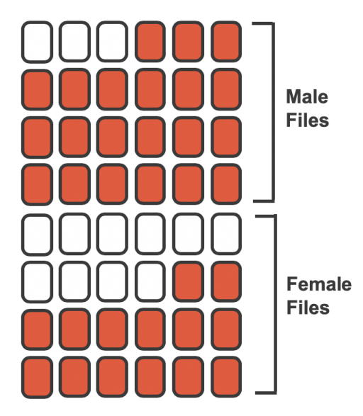
We have 48 files: 24 were labelled ‘female’ (bottom 24) and 24 were labelled ‘male’ (top 24). Of these cards, 35 were ‘promoted’ (red) and 13 were ‘not promoted’ (white).

Variability of the Statistic, Under the Assumption

If the decision of the supervisors was independent of the gender of the applicant file, then the results we obtained were entirely due to chance. The files were all identical aside from the declared name/gender of the applicant, so we assume that each supervisor would have made the same decision regardless of the file presented.

We can use randomization to explore this scenario.

Randomization: Decision Independent of Gender

We can perform a randomization simulation, where we simulate what could have happened, under the scenario just mentioned. In such a simulation, we shuffle the 48 files (35 labelled as ‘promoted’ and 13 labelled as ‘not promoted’) and deal them out into two stacks: 24 into a pile labelled ‘female’ and 24 into a pile labelled ‘male’.

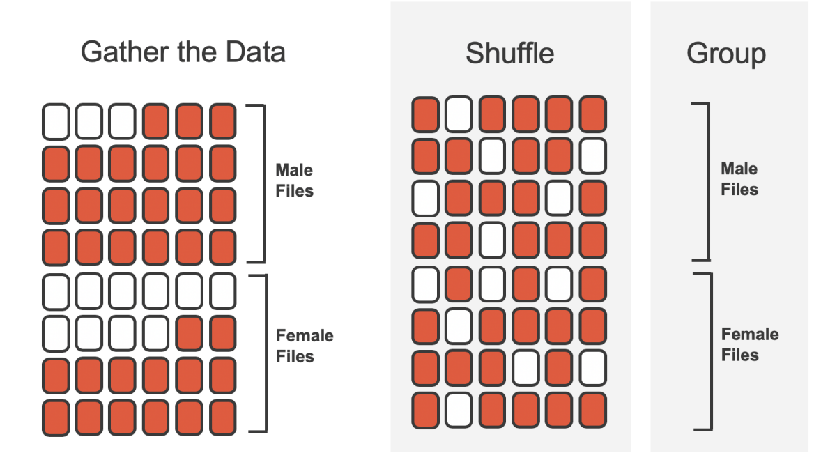
Variability of the Statistic

Even if the two are independent, we won’t expect the difference in the proportions to be exactly 0. For one thing, we have 35 ‘promoted’ cases, which we can’t divide evenly into two groups. So no matter what, there will be some difference in the two arbitrary (gender) groups.

How much variability is a sign of something suspicious going on?

That’s the point of statistics!

Stating the Hypotheses

\(H_0\): Null hypothesis. The variables gender and decision are independent. The difference in promotion rates of 29.2% was due to natural variability inherent in the population.
\(H_A\): Alternative hypothesis. The variables gender and decision are not independent. The difference in promotion rates of 29.2% was not due to natural variability, and equally qualified female personnel are less likely to be promoted than male personnel.

Simulation 1

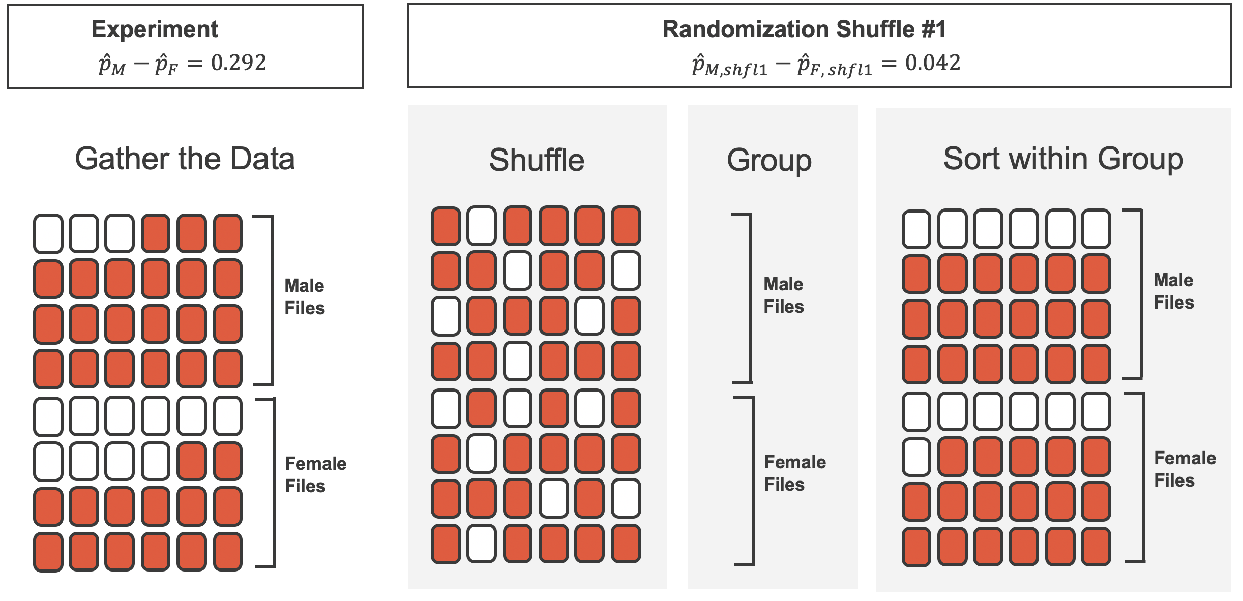
Simulation 1: Summary

	Promoted
	Yes	No	Total
Gender
Male	18	6	24
Female	17	7	24
Total
	35	13	48

Difference: 18/24 - 17/24 = 0.0417.

Doing the Simulation Again and Again

So we did one simulation, and found a really small difference in promoted proportions, under the assumption that there is independence. Is this evidence?

Do it again!

Simulation 2: difference of -0.0417
Simulation 3: difference of 0.208
…. ? COMPUTERS!

Results of 100 Shuffles

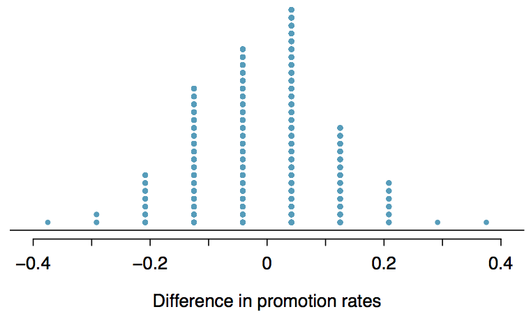
Figure: Stacked dot plot of differences from 100 simulations under assumption of independence.

What was our observed statistic again? 0.292

So Are Our Data Weird?

The question we can answer, at the end of all of this, is:

How often would we see a result like 0.292, or even bigger?

And the answer is: around 2 times in 100 simulations.

Is This Rare?

The difference of 29.2% is a rare event if there really is no impact from listing gender in the candidates’ files, which provides us with two possible interpretations of the study results:

If \(H_0\), the Null hypothesis, is true: gender has no effect on promotion decision, and we observed a difference that is so large that it would only happen rarely.
If \(H_A\), the Alternative hypothesis, is true: gender has an effect on promotion decision, and what we observed was actually due to equally qualified female candidates being discriminated against in promotion decisions, which explains the large difference of 29.2%.

In our analysis, we determined that there was only approximately a 0.02 (2%) probability of obtaining a sample where 29.2% or more male candidates than female candidates get promoted under the null hypothesis, so we conclude that the data provide strong evidence of gender discrimination against female candidates by the male supervisors. In this case, we would side with the \(H_A\), alternative hypothesis, as a more plausible outcome.

Statistical Inference: Definition

Statistical inference is the practice of making decisions and conclusions from data in the context of uncertainty. Errors do occur, just like rare events, and the dataset at hand might lead us to the wrong conclusion.

While a given dataset may not always lead us to a correct conclusion, statistical inference gives us tools to control and evaluate how often these errors occur.

Re-Doing the Gender Discrimination Example

Earlier, we “did” a simulation where we just showed you the results. Now we’re going to do the entire simulation, properly, and then add up the results manually (in code). We will use pipes along with a new package, infer, that allows us to build hypothesis tests in the same way that we build ggplots.

library(dplyr)
library(infer)
library(openintro)
data(gender_discrimination)
gender_discrimination |> glimpse()

Rows: 48
Columns: 2
$ gender   <fct> male, male, male, male, male, male, male, male, male, male, m…
$ decision <fct> promoted, promoted, promoted, promoted, promoted, promoted, p…

Re-Doing the Gender Discrimination Example

Now, let’s pipe the data.frame into a specification, then establish our null hypothesis (independence), and generate permutation results.

set.seed(15)
gender_discrimination_perm3 <- gender_discrimination |> 
  specify(decision ~ gender, success = "promoted") |>
  hypothesize(null = "independence") |>
  generate(reps = 3, type = "permute")

gender_discrimination_perm3 |> glimpse()

Re-Doing the Gender Discrimination Example

Rows: 144
Columns: 3
Groups: replicate [3]
$ decision  <fct> promoted, not promoted, not promoted, promoted, promoted, pr…
$ gender    <fct> male, male, male, male, male, male, male, male, male, male, …
$ replicate <int> 1, 1, 1, 1, 1, 1, 1, 1, 1, 1, 1, 1, 1, 1, 1, 1, 1, 1, 1, 1, …

(why 144 rows? \(48 \times 3\))

Re-Doing the Gender Discrimination Example

We can then group these by replicate, and count the results:

gender_discrimination_perm3 |>
  group_by(replicate) |>
  count(gender, decision)

# A tibble: 12 × 4
# Groups:   replicate [3]
   replicate gender decision         n
       <int> <fct>  <fct>        <int>
 1         1 male   promoted        17
 2         1 male   not promoted     7
 3         1 female promoted        18
 4         1 female not promoted     6
 5         2 male   promoted        19
 6         2 male   not promoted     5
 7         2 female promoted        16
 8         2 female not promoted     8
 9         3 male   promoted        19
10         3 male   not promoted     5
11         3 female promoted        16
12         3 female not promoted     8

Re-Doing the Gender Discrimination Example

Finally, calculate the difference in proportion, male - female

diffs <- gender_discrimination_perm3 |>
  calculate(stat = "diff in props", order = c("male", "female"))
diffs

Response: decision (factor)
Explanatory: gender (factor)
Null Hypothesis: ind...
# A tibble: 3 × 2
  replicate    stat
      <int>   <dbl>
1         1 -0.0417
2         2  0.125 
3         3  0.125

Re-Doing the Gender Discrimination Example

Then our observed statistic used the breakdown of 21 / 24 and 14 / 24. How often do we see a result this big, or bigger?

observed <- gender_discrimination |>
  observe(decision ~ gender, success = "promoted", 
          stat = "diff in props", order = c("male", "female")) |>
  pull(stat)

perm_diffs <- diffs |> pull(stat)
perm_diffs

[1] -0.04166667  0.12500000  0.12500000

perm_diffs >= observed

[1] FALSE FALSE FALSE

sum(perm_diffs >= observed)

[1] 0

Re-Doing, Bigger, without the manual steps

set.seed(12)
results  <- gender_discrimination |> 
  specify(decision ~ gender, success = "promoted") |>
  hypothesize(null = "independence") |>
  generate(reps = 100, type = "permute") |>
  calculate(stat = "diff in props", order = c("male", "female")) |>
  count(as_extreme = stat >= observed)
results

Response: decision (factor)
Explanatory: gender (factor)
Null Hypothesis: ind...
# A tibble: 2 × 2
  as_extreme     n
  <lgl>      <int>
1 FALSE         99
2 TRUE           1

Re-Doing, Bigger(er)

set.seed(12)
results  <- gender_discrimination |> 
  specify(decision ~ gender, success = "promoted") |>
  hypothesize(null = "independence") |>
  generate(reps = 10000, type = "permute") |>
  calculate(stat = "diff in props", order = c("male", "female")) |>
  count(as_extreme = stat >= observed)
results

Response: decision (factor)
Explanatory: gender (factor)
Null Hypothesis: ind...
# A tibble: 2 × 2
  as_extreme     n
  <lgl>      <int>
1 FALSE       9745
2 TRUE         255

So in 10,000 replicates of this shuffling simulation, we saw a result like our observed statistic around 2.55% of the time. Not very likely!

Recap

We’ve spent today developing the general framework for hypothesis testing.
We looked at an example of two proportions.
We will continue this development in the coming lectures.

Readings for Today

Today’s topic was drawn from Chapter 11 of Introduction to Modern Statistics (2e).