A Bernoulli trial is one of the simplest distributions – it has two possible outcomes:
success
failure
Example 1: Flipping a coin where getting a heads is a “success” and tails is “failure”.
Example 2: Check a tire to see if it is flat (“success”), or inflated (“failure”).
Distribution of a Bernoulli R.V.
The distribution (sometimes called a Probability Mass Function) of a Bernoulli random variable (R.V.) is:
\[
P(X = x) = p(x) = \begin{cases}1 - p & \text{if } x = 0 \\
p & \text{if } x = 1 \\
0 & \text{else}
\end{cases}
\]
So two cases: “success” (probability \(p\)) and “failure” (probability \(1-p\)).
This is the mathematical model for our simplest probability example: coin flips! This is general enough to allow for non-fair coins - the probability of heads does not have to be the same as the probability of tails. They just have to add up to 1.
Binomial Distribution
A very important discrete distribution is the binomial distribution, which results when we have:
a fixed number of trials, \(n\)
only two outcomes possible in each trial
each trial is independent
the probability of a success is the same on each trial
Definition: the binomial distribution counts the number of successes in \(n\) independent trials of an experiment with fixed probability of success, \(p\). In other words, a binomial is what happens when we have a number \(n\) of independent Bernoulli trials.
Binomial Notation
If \(X\) is a Binomial random variable then we would use the notation:
\[
X \sim \text{Binomial}(n, p)
\]
\(n\) - the fixed number of trials/experiments
\(x\) - a specific number of successes we are interested in (must be between \(0\) and \(n\), obviously)
\(p\) - probability of success in any one trial/experiment
\(P(X = x)\) - the probability of getting exactly \(x\) successes in \(n\) trials
Things To Be Cautious Of
make sure that \(x\) and \(p\) are referring to the same event as “success” (remember, just a label)
make sure that all trials/experiments are independent
when sampling without replacement, make sure your total number of trials/experiments is small when compared to population
independence!
Example 1
Suppose you have no idea how to answer the questions on a True/False test with 10 questions, and you decide to just flip a coin for each one. You then count how many questions you actually got correct.
\(x =\) number of questions correct
\(n = 10\)
\(p = 0.5\) (fair coin?)
trials are independent, since the coin flips have nothing to do with one another
In this situation, what is the probability of getting at least 6/10?
Example 2
According to Statistics Canada, as of the last census in 2016, 86.3% of Canadians between the ages of 25 and 64 have a completed high school diploma, or equivalent. If we randomly select 15 Canadians aged 25-64, what is the probability distribution of the number of sampled people who have completed a high school diploma?
Find the probability that at least 8 out of 15 randomly selected Canadians aged 25-64 will have such a diploma.
R Syntax for Computing Things with Binomials
Example:
sum( dbinom(x =0:6, size =10, prob =0.5) )
[1] 0.828125
This gives the probability of getting six or less correct answers in ten trials, with a 50/50 probability (like Example 1).
R Syntax for Computing Things with Binomials
Example:
sum( dbinom(x =7:10, size =10, prob =0.5) )
[1] 0.171875
This gives the probability of getting MORE THAN SIX correct answers in ten trials, again with a 50/50 probability (like Example 1).
Note: this is not “greater than or equal to”, it is strictly greater than 6.
General R Syntax
For the probability associated with a specific number of successes:
dbinom(x = [specific successes interested in],size = [total number of trials],prob = [probability of success in each trial])
For the probability associated with observing one of a set of successes:
sum( dbinom(x = [set of successes interested in],size = [total number of trials],prob = [probability of success in each trial]) )
We would use a vector to represent the “set of successes”.
Either c(1,9,10) or, if we have a sequence of successes, 3:6.
OR, both! c(1, 3, 8:10)
Families of Continuous Distributions
Continuous distributions
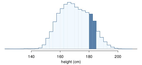
Below is a histogram of the distribution of heights of US adults.
The proportion of data that falls in the shaded bins gives the probability that a randomly sampled US adult is between 180 cm and 185 cm (about 5’11” to 6’1”).
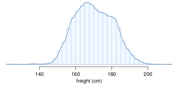
From histograms to continuous distributions
Since height is a continuous numerical variable, its probability density function is a smooth curve. We’re not all rounded exact cm in height. I might be 172.143cm, and you might be 172.196cm, but on this graph, we’d be the same rectangle.
Probabilities from continuous distributions
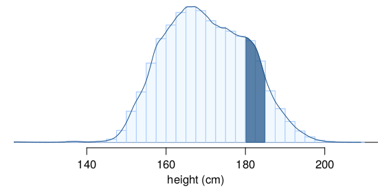
Therefore, the probability that a randomly sampled US adult is between 180 cm and 185 cm can also be estimated as the shaded area under the curve.
Important
This is an incredibly important idea. There are two probabilities here: the discrete estimate, computed using the areas of the rectangles and summing; and the continuous estimate, computed using calculus.
By definition… (REALLY IMPORTANT)
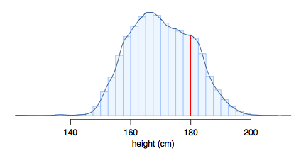
Since continuous probabilities are estimated as “the area under the curve”, the probability of a person being exactly 180 cm (or any exact value) is defined as 0.
The Normal Distribution
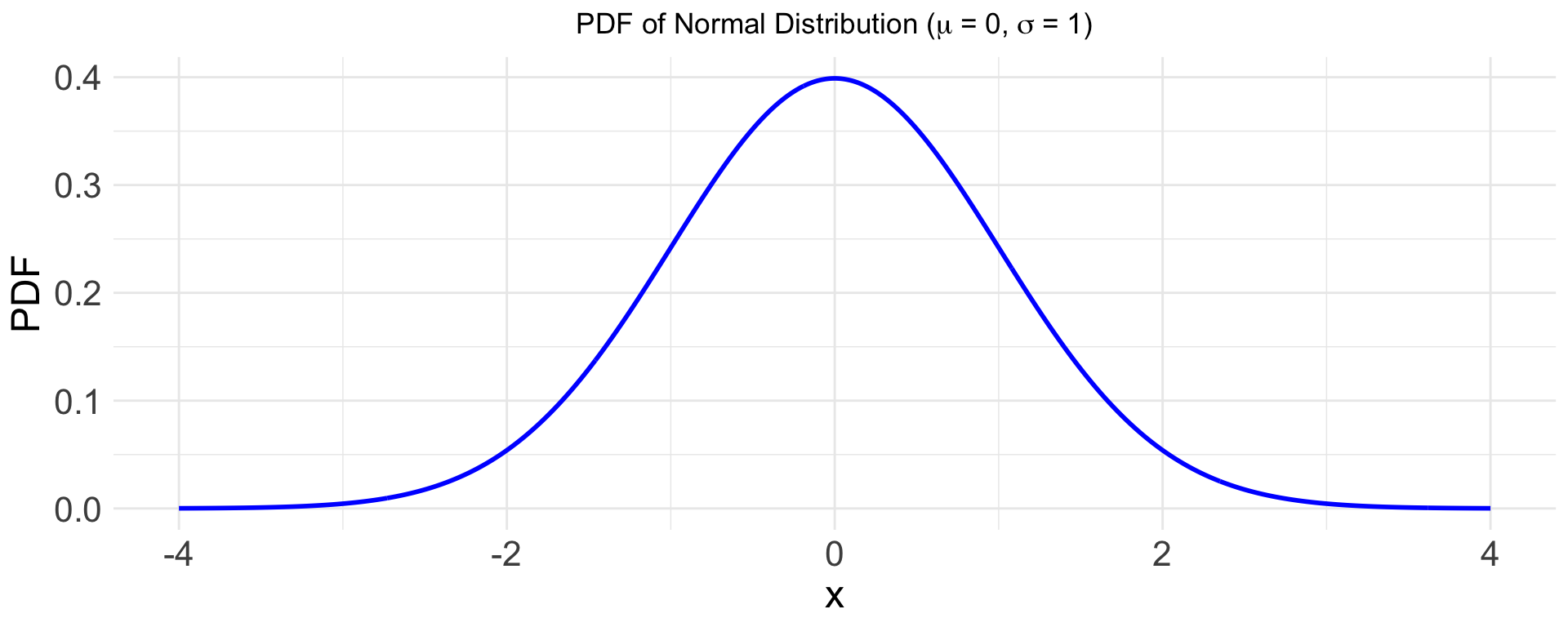
Unimodal and symmetric, bell shaped curve
Many variables are nearly normal, but none are exactly normal
Denoted as \(\mathcal{N}(\mu, \sigma) \rightarrow\) Normal with mean \(\mu\) and standard deviation \(\sigma\)
Very important for theoretical work; we won’t use it much
Heights of Males
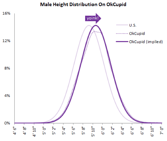
“The male heights on OkCupid very nearly follow the expected normal distribution – except the whole thing is shifted to the right of where it should be. Almost universally guys like to add a couple inches.”
“You can also see a more subtle vanity at work: starting at roughly 5’8”, the top of the dotted curve tilts even further rightward. This means that guys as they get closer to six feet round up a bit more than usual, stretching for that coveted psychological benchmark.”1
Heights of Females
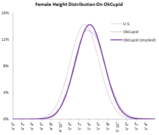
“When we looked into the data for women, we were surprised to see height exaggeration was just as widespread, though without the lurch towards a benchmark height.”1
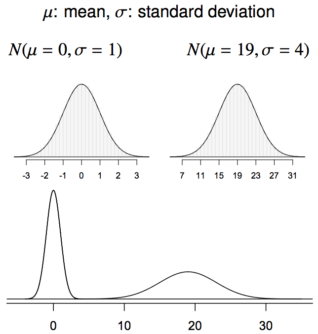
Normal distributions with different parameters
Percentiles
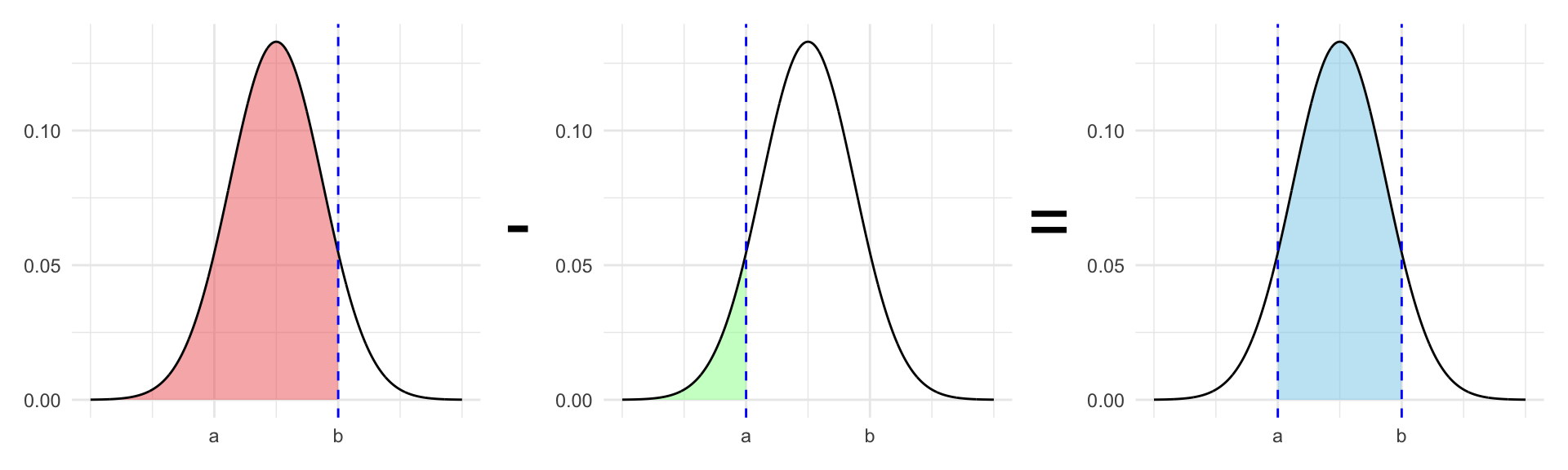
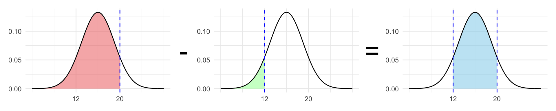
Percentile is the percentage (proportion) of observations that fall below a given data point
Graphically, percentile is the area under the probability distribution curve to the left of that observation
Think about the two questions we can ask from the diagram below
Working with Normal RVs in R
When \(X\) is a normally distributed random variable with mean \(\mu\) and standard deviation \(\sigma\), we would write:
\[
X \sim N(\mu, \sigma)
\]
The basic probability expressions that we can calculate in R are: \[
\text{Find Probabilities:} \quad\qquad P(X \leq q) \quad \text{or} \quad P(X > q)
\]
Assuming \[
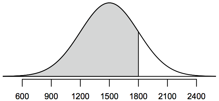
X \sim N(\mu = 1500, \sigma = 300)
\] We could find: \[
P(X < 1800)
\]R:
pnorm(1800, mean =1500, sd =300)
[1] 0.8413447
Example: Quality Control
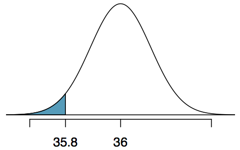
At the Heinz ketchup factory, the amounts which go into bottles of ketchup are supposed to be normally distributed with mean 36 oz. and standard deviation 0.11 oz. Once every 30 minutes a bottle is selected from the production line, and its contents are noted precisely. If the amount of ketchup in the bottle is below 35.8 oz. or above 36.2 oz., then the bottle fails the quality control inspection. What percent of bottles have less than 35.8 ounces of ketchup?
Let \(X\) = amount of ketchup in a bottle: \(X \sim \mathcal{N}(\mu = 36, \sigma = 0.11)\)
Finding the exact probability - using R
We have that \(X\) is the amount of ketchup in a bottle where \[
X \sim \mathcal{N}(\mu = 36, \sigma = 0.11)
\]
Then, we want to find: \[
P(X < 35.8)
\]
Finding the exact probability - using R
We have that \(X\) is the amount of ketchup in a bottle where \[
X \sim \mathcal{N}(\mu = 36, \sigma = 0.11)
\]
Then, we want to find: \[
P(X < 35.8)
\]
pnorm(q =35.8, mean =36, sd =0.11, lower.tail =TRUE)
[1] 0.03451817
Recap: Normal Distribution
The normal distribution is the most famous distribution in statistics. However, it’s also one of the most error-prone. We will not use it directly in very many places.
Instead, we will use the distribution we’ll talk about next most of the time. For this course, MATH 1051H, there are actually only two distributions we care about:
the binomial distribution
the t distribution (coming up soon, not this week!)
In MATH 1052H you’ll also spend some time using the:
F distribution
\(\chi^2\) distribution
Computing Areas Under the Curve
Using the Normal
We said earlier today that the normal isn’t actually something we’ll spend a lot of time on. And this is true.
However, it’s a very common distribution, and it makes a good teaching tool.
So for the rest of today, we’re going to do some examples using the normal distribution, where we compute the area under the curve and evaluate the probabilities.
The logic will translate nicely to the other cases, and we’ll look at those next week.
Discrete RVs
Continous RVs
“Space” between values
\(\infty\) number of values in any interval
\(P(X = x) = p(x)\);
\(P(X = x) = 0\)
\(P(X \leq x) =\) a sum of values
\(P(X \leq x) =\) area under \(f(x)\) to left of \(x\)
sum(dbinom(x, size, prob))
pnorm(x, mean, sd)
Formula to Calculate Probabilities
For any Normally distributed RV, \(X\).
\[
X \sim N(\mu = m, \sigma = s)
\]
In R,
pnorm(q, m, s, lower.tail = TRUE)
you have q; it calculates \(P(X \leq q)\)
qnorm(p, m, s, lower.tail = TRUE)
you have \(P(X \leq q)\), it finds you \(q\)
Formula to Calculate Probabilities
For any Normally distributed RV, \(X\). You have (or want)
\[
P(X > q)
\]
In R,
pnorm(q, m, s, lower.tail = FALSE)
you have q; it calculates \(P(X > q)\)
qnorm(p, m, s, lower.tail = FALSE)
you have \(P(X > q)\), it finds you \(q\)
Fun Facts For Continuous Distributions (like Normal):
Given a distribution, like the normal, we can find the “area under the curve”, which is a probability.
This is very important for most of the rest of the semester (and for 1052H), as a lot of problems (after dealing with word problem translation and math) turn into a final part which is “compute a probability”.
We will practice these techniques a lot in the coming weeks.
Finally: Inverse Problems
Finding Quantiles from Probabilities
In the previous slides we were finding probabilities from quantiles \[
P(X \leq x) = {\color{red}p}
\]
The inverse problem is also interesting: given a probability (area!), what must the cutoff(s) have been to make that work?
The functions to do this in R are quantile functions (q), e.g., qnorm(p = prob, mean = m, sd = s)
Note
Inverse functionsundo the effect of the original function. E.g., \(f(x) = 2x\) and \(f^{-1}(x) = x/2\) then we would have: \(f^{-1}(f(x)) = x\)
Consider:
qnorm(pnorm(15, mean = mean, sd = sd), mean = mean, sd = sd)
[1] 15
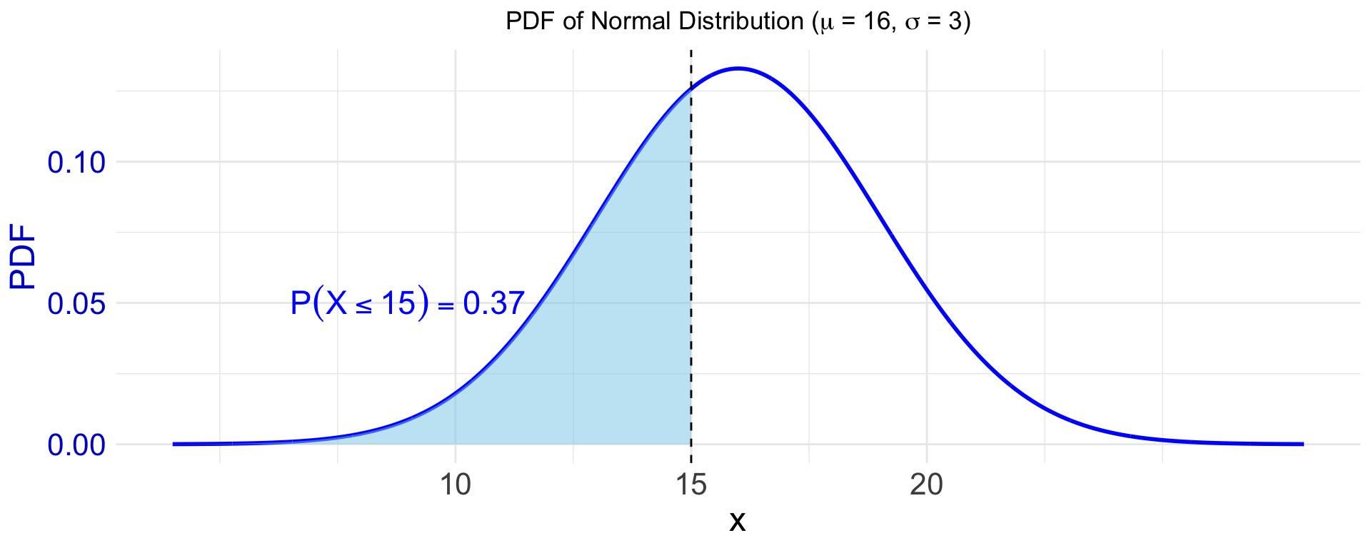
e.g., qnorm for \(P(X \leq x) = 0.37\)
pnorm(q =15.0, mean = mean, sd = sd)
[1] 0.3694413
qnorm(p =0.3694, mean = mean, sd = sd)
[1] 14.99967
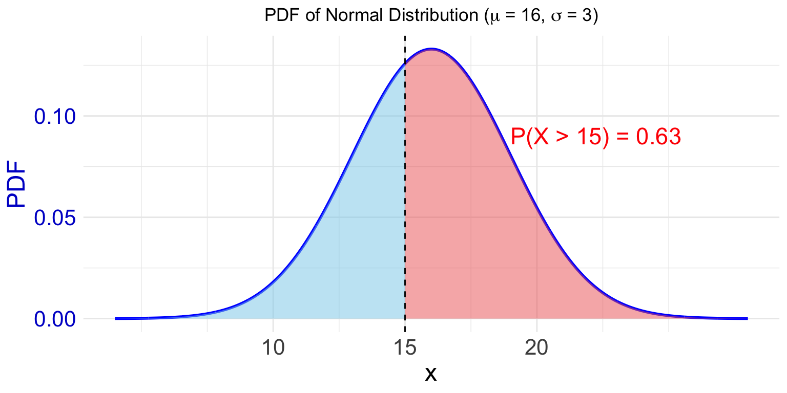
e.g., qnorm for \(P(X > x) = 0.63\)
qnorm(0.63, mean = mean, sd = sd, lower.tail =FALSE)
[1] 15.00444
qnorm(1-0.63, mean = mean, sd = sd, lower.tail =TRUE)
[1] 15.00444
To Come
Next week, we will continue working with these ideas. It’s secretly integration (shhhh!) … but this is a non-calculus course, so we’re just going to say “Heyyyy, computer! Do this for me!” and if we do it just right, our computers will compute the integrals (“area under the curves”) for us!
We’ve done all our examples with normals so far, and will continue to do so on Friday, but next week we’re going to expand the ideas into a couple of other directions, as setup for our first major topic of statistics.