Now the variable names are the whole question, so let’s shorten those:
coffee <- coffee |>rename(coffee =`How much coffee do you drink per day on average? (Answer your best guess in millilitres)`,sleep =`How much sleep do you get on average? (Answer your best guess in minutes)`) |>select(coffee, sleep)
And I do some final cleaning (details not important):
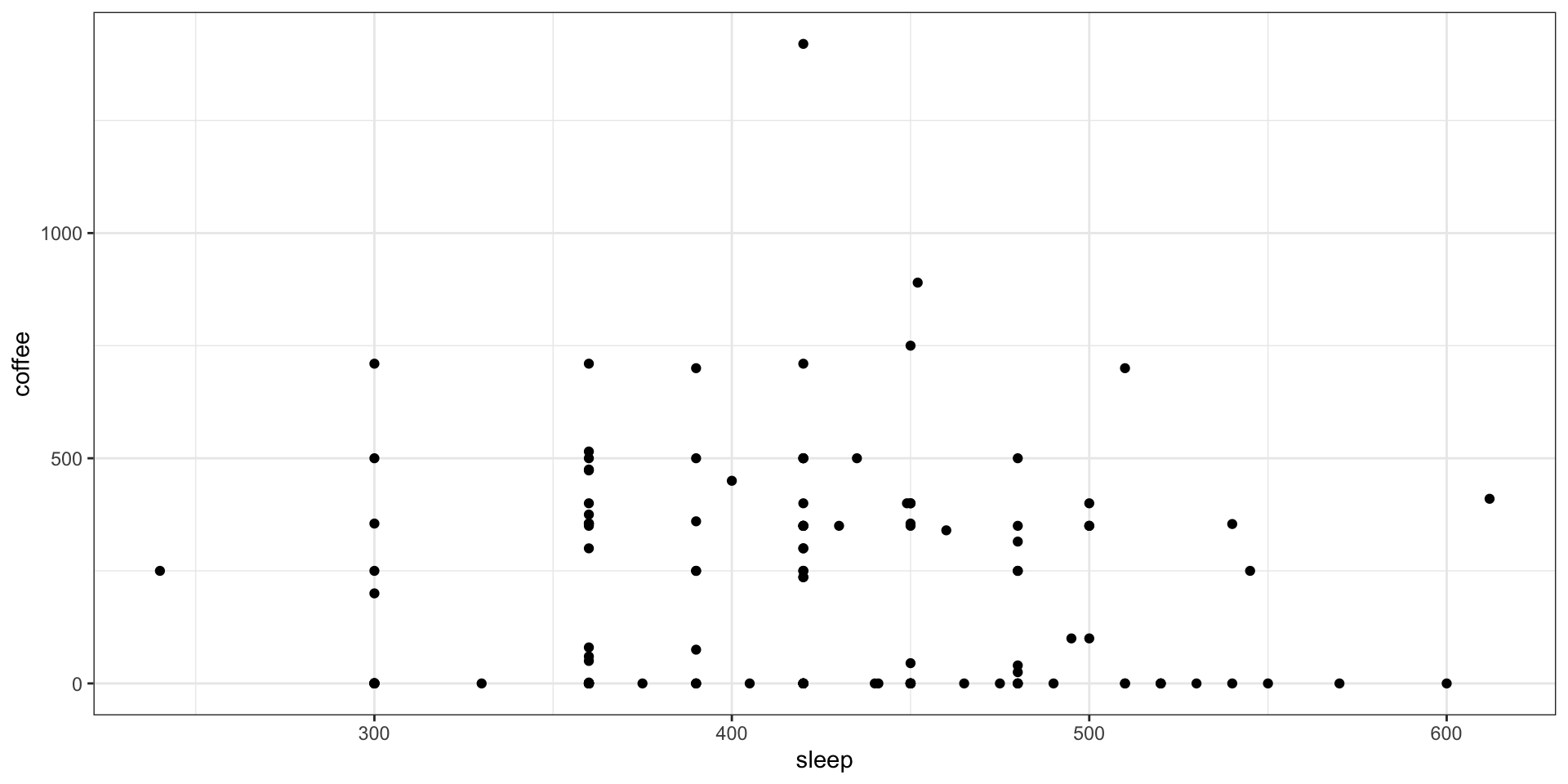
Unfortunately, this is not a great example of a linear relationship for the rest of our slides, so we’ll have to go back to our poverty example.
But, let’s try again before Monday’s class
Let’s Do More Science! (Homework)
We are going to investigate whether there is a linear relationship between the number of chapters in a book and the number of pages in the book.
Please choose any book you have access to. It can be a textbook, novel, nonfiction book, cookbook, graphic novel, etc.
Deadline: Friday at Noon
You may submit data for as many different books as you like, but each submission should represent a different book.
For each book, enter: the number of chapters; the number of pages; the name of book.
This activity is not required, but it’s a fun way to make some data to use on Monday.
Fitting a line by least squares regression
The Idea
We want to fit a straight line of the form: \[
\hat{y} = b_0 + b_1 x
\]
This line should be as “close” to each point as possible.
How do we define “close” ?
The model we will use is: \[
Y_i = \beta_{0} + \beta_{1}x_i + \epsilon_{i}
\]
The Data
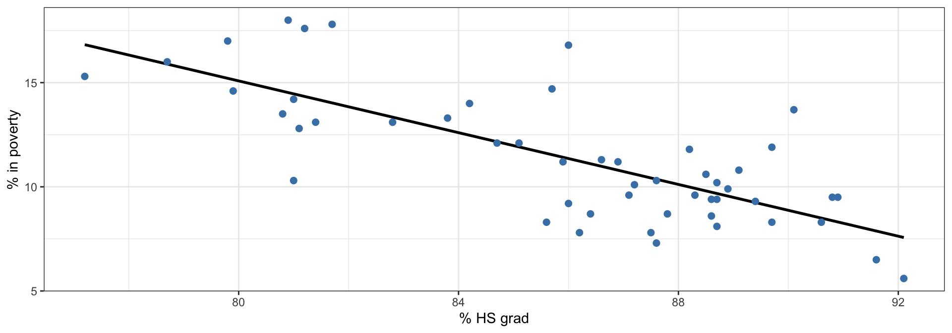
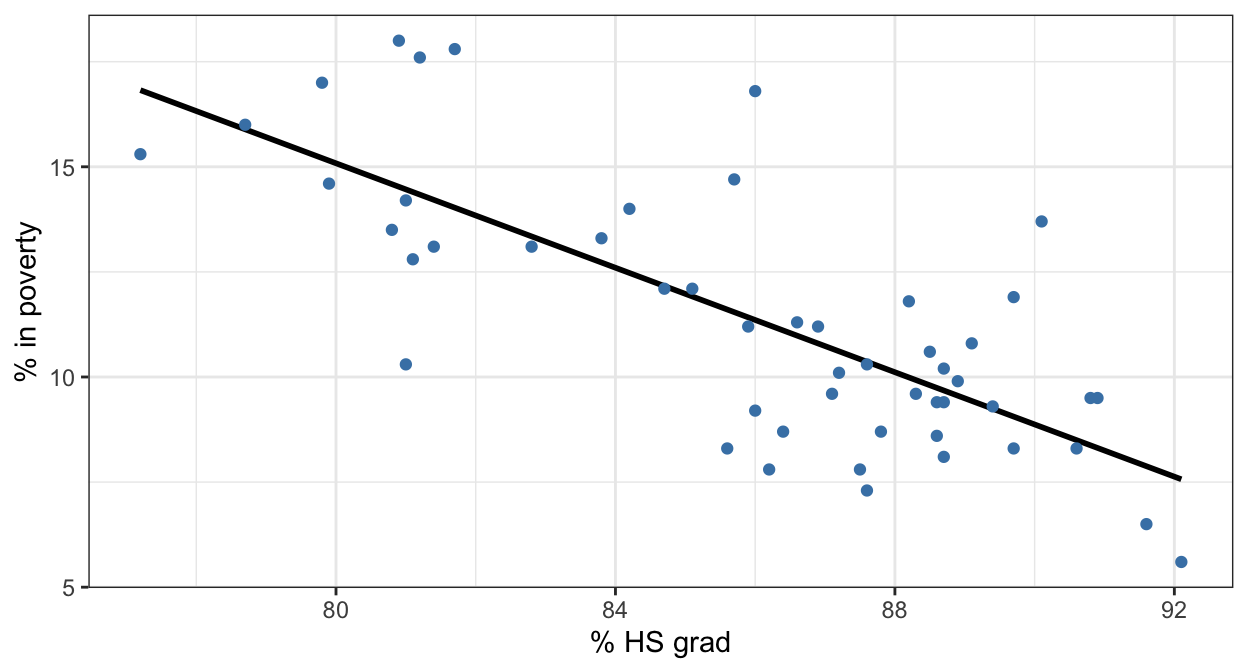
We have data from 50 states (plus DC) on poverty and high school graduation rates.
The black line is the “best” line that describes the relationship.
How do we calculate this line?
Residuals
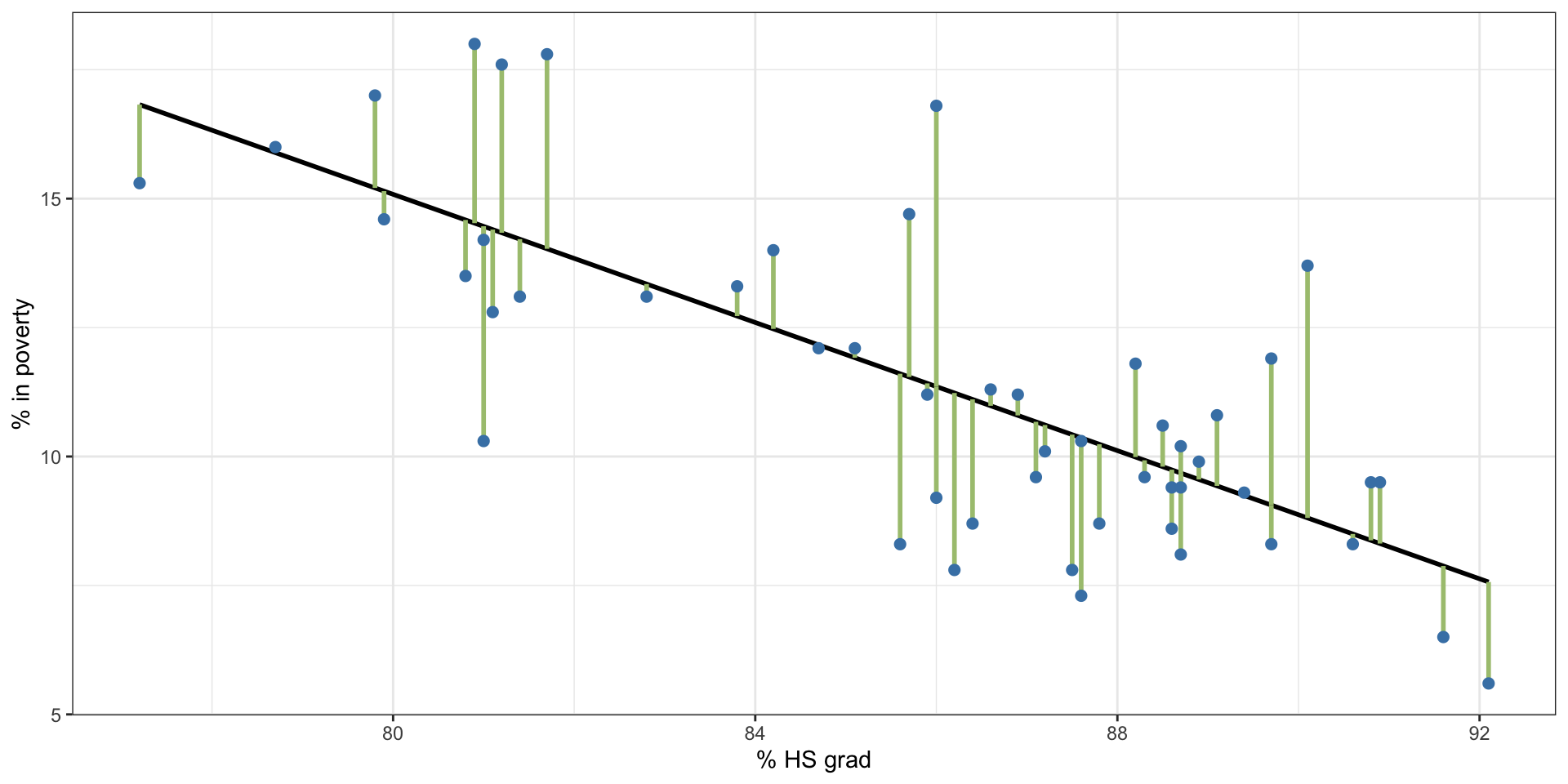
Residuals are the leftovers from the model fit: Data = Fit + Residual
Residuals (cont.)
Formally, residuals are the difference between the observed values of the response (\(y_i\)) and predicted values of the response from the model (\(\hat{y}_i\)).
\[
e_i = y_i - \hat{y}_i
\]
Specific Residuals
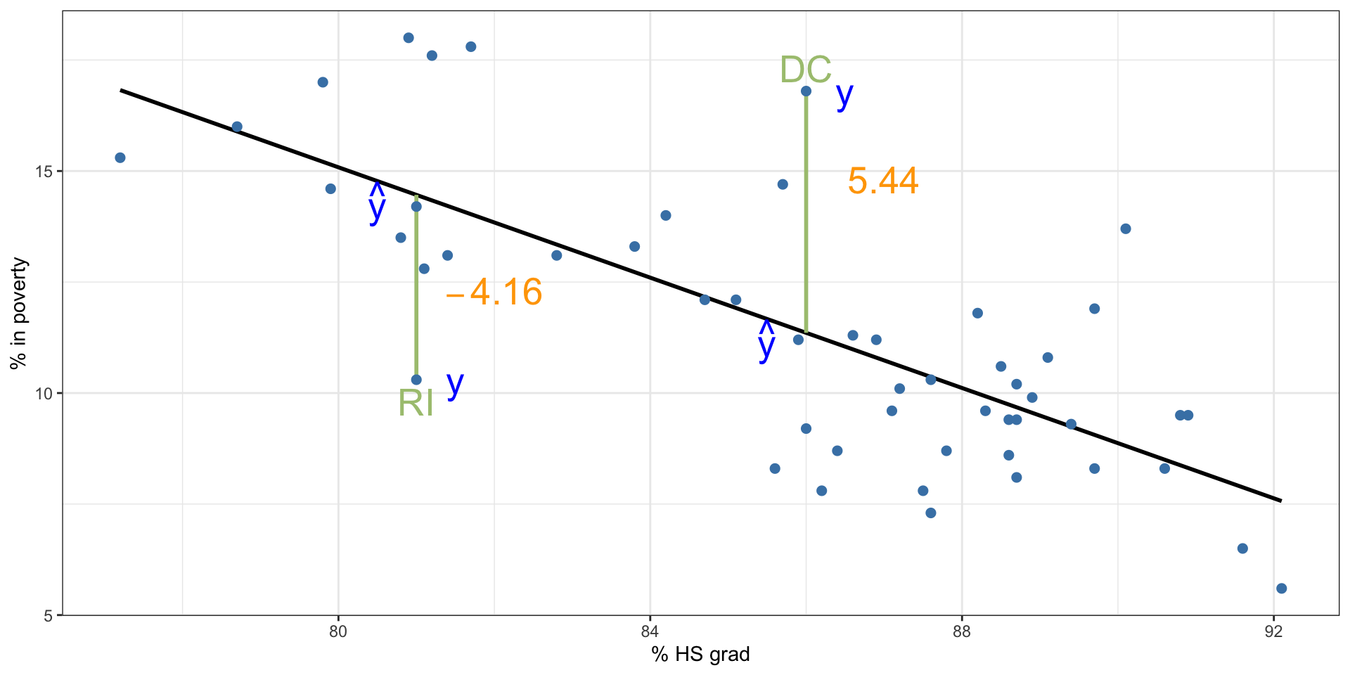
% living in poverty in DC is 5.44% more than predicted.
% living in poverty in RI is 4.16% less than predicted.
A measure for the best line
What is “close”?
We want a line that has small residuals:
Option 1: Minimize the sum of magnitudes (absolute values) of residuals \[
|e_1| + |e_2| + \cdots + |e_n|
\]
Option 2: Minimize the sum of squared residuals – known as least squares\[
e_1^2 + e_2^2 + \cdots + e_n^2
\]
Option 3 … 100: actual topics of research!
Why least squares?
Under the assumption that \(\epsilon_{i} \overset{\text{iid}}{\sim} N(\mu, \sigma_{\epsilon})\), the least-squares estimates are maximum likelihood!
Most commonly used
Easier to compute by hand and using software
In many applications, a residual twice as large as another is usually more than twice as bad
The least squares line
\[
\hat{y} = \beta_0 + \beta_1 x
\]
Notation:
Intercept:
Parameter: \(\beta_0\)
Point estimate: \(b_0\)
Slope:
Parameter: \(\beta_1\)
Point estimate: \(b_1\)
The least squares line
mod <-lm(Poverty ~ Graduates, data = poverty)summary(mod)
Call:
lm(formula = Poverty ~ Graduates, data = poverty)

Residuals:
    Min      1Q  Median      3Q     Max
-4.1624 -1.2593 -0.2184  0.9611  5.4437

Coefficients:
            Estimate Std. Error t value Pr(>|t|)
(Intercept) 64.78097    6.80260   9.523 9.94e-13 ***
Graduates   -0.62122    0.07902  -7.862 3.11e-10 ***
---
Signif. codes:  0 '***' 0.001 '**' 0.01 '*' 0.05 '.' 0.1 ' ' 1

Residual standard error: 2.082 on 49 degrees of freedom
Multiple R-squared:  0.5578,    Adjusted R-squared:  0.5488
F-statistic: 61.81 on 1 and 49 DF,  p-value: 3.109e-10
Slope
The slope of the regression can be calculated as \[
b_1 = \frac{s_y}{s_x} R
\]
but we will just use R, and identify it from the summary table:
mod |>coefficients()
(Intercept)   Graduates
 64.7809658  -0.6212167
(so \(b_1 = -0.62\))
Interpretation For each additional % point in HS graduate rate, we would expect the % living in poverty to be lower on average by 0.62% points.
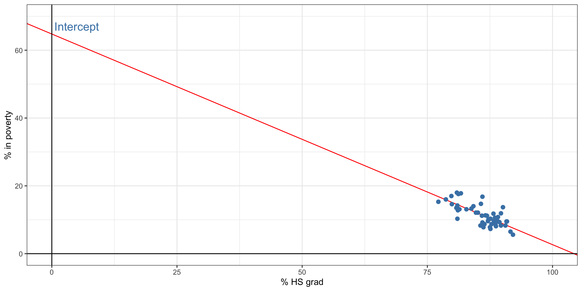
Intercept
The intercept is where the regression line intersects the \(y\)-axis. The calculation of the intercept uses the fact the regression line always passes through \((\bar{x},\bar{y})\):
\[
b_0 = \bar{y} - b_1 \bar{x},
\]
but again, we will just use R and identify it:
mod |>coefficients()
(Intercept)   Graduates
 64.7809658  -0.6212167
(so \(b_0 = 64.78\)).
Intercept
\(\;\)
Which of the following is the correct interpretation of the intercept?
For each % point increase in HS graduate rate, % living in poverty is expected to increase on average by 64.68%.
For each % point decrease in HS graduate rate, % living in poverty is expected to increase on average by 64.68%.
Having no HS graduates leads to 64.68% of residents living below the poverty line.
States with no HS graduates are expected on average to have 64.68% of residents living below the poverty line.
In states with no HS graduates % living in poverty is expected to increase on average by 64.68%.
More on the intercept
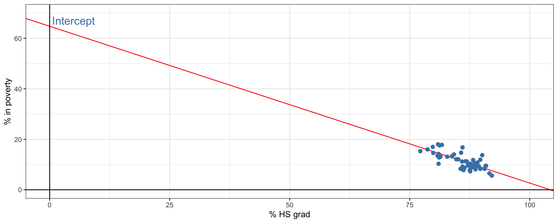
Since there are no states in the dataset with no HS graduates, the intercept is of no interest, not very useful, and also not reliable since the predicted value of the intercept is so far from the bulk of the data.
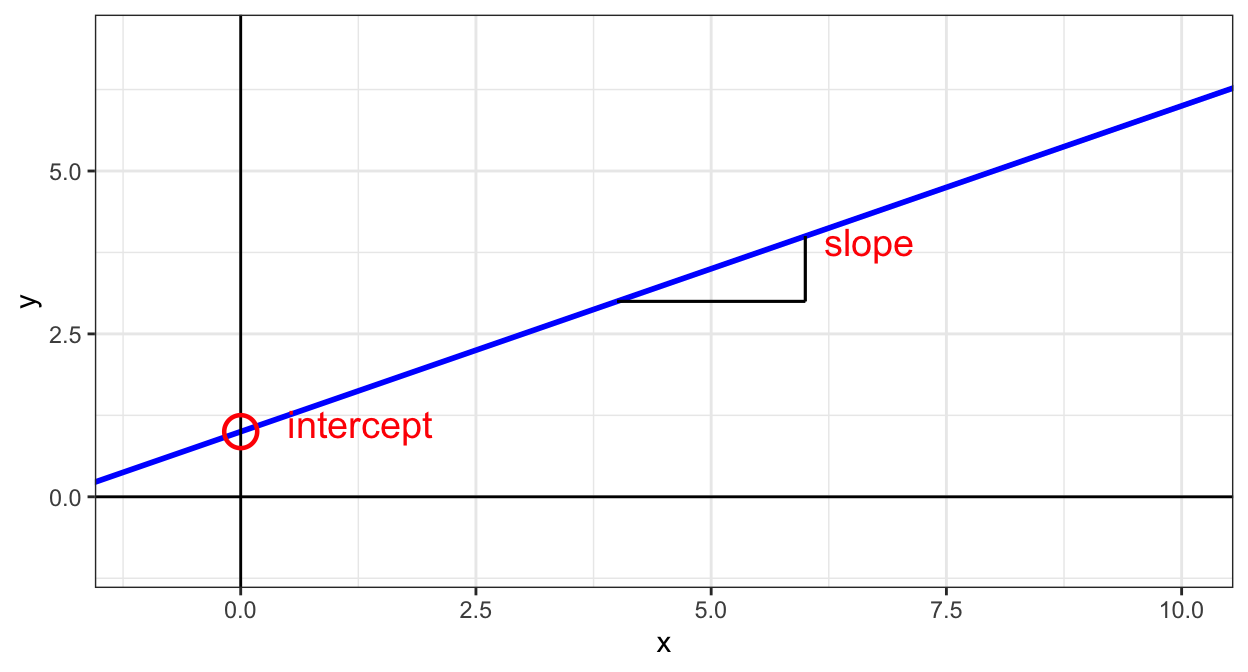
Intercept: When \(x = 0\), \(y\) is expected to equal the intercept.
Slope: For each unit in \(x\), \(y\) is expected to increase / decrease on average by the slope.
These statements are not causal, unless the study is a randomized controlled experiment.
Prediction & extrapolation
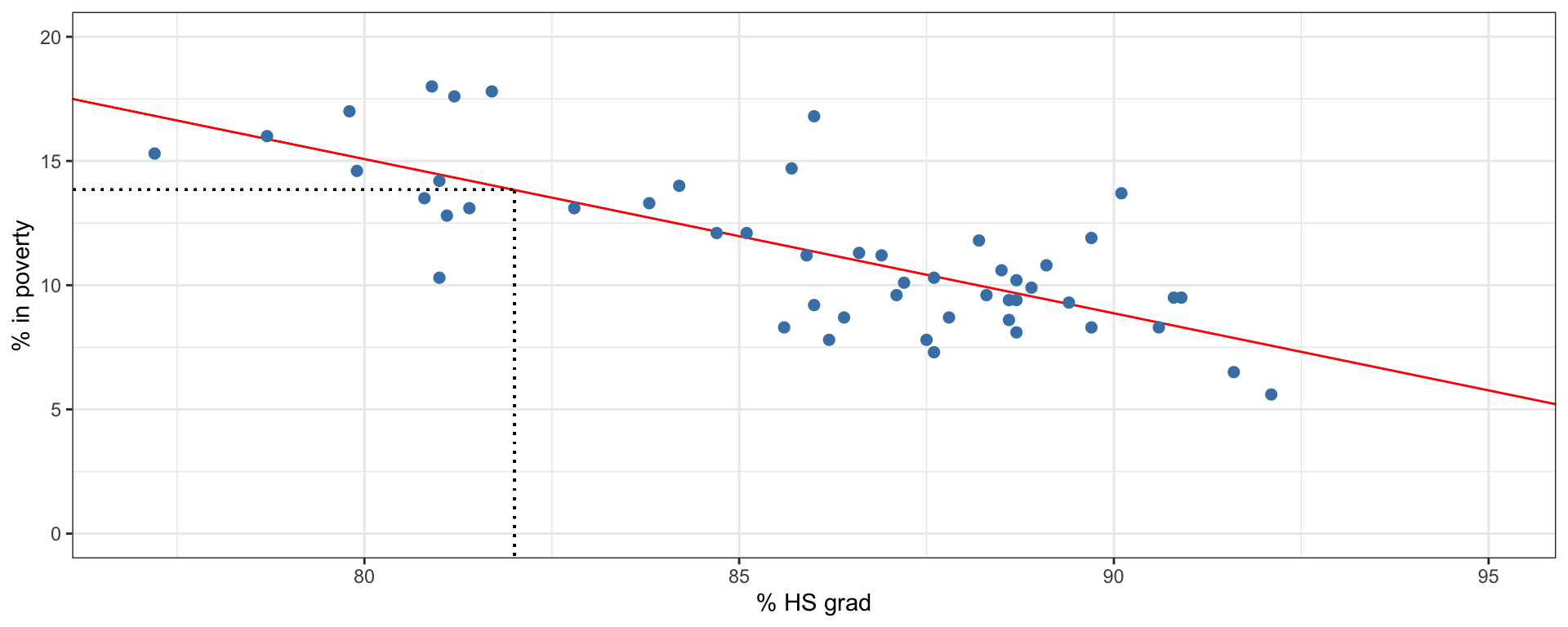
Prediction
Using the linear model to predict the value of the response variable for a given value of the explanatory variable is called prediction, simply by plugging in the value of \(x\) in the linear model equation.
There will be some uncertainty associated with the predicted value.
Extrapolation
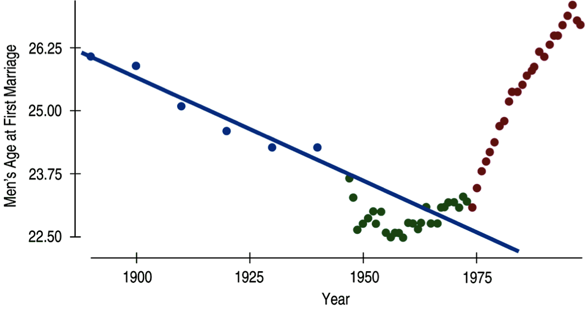
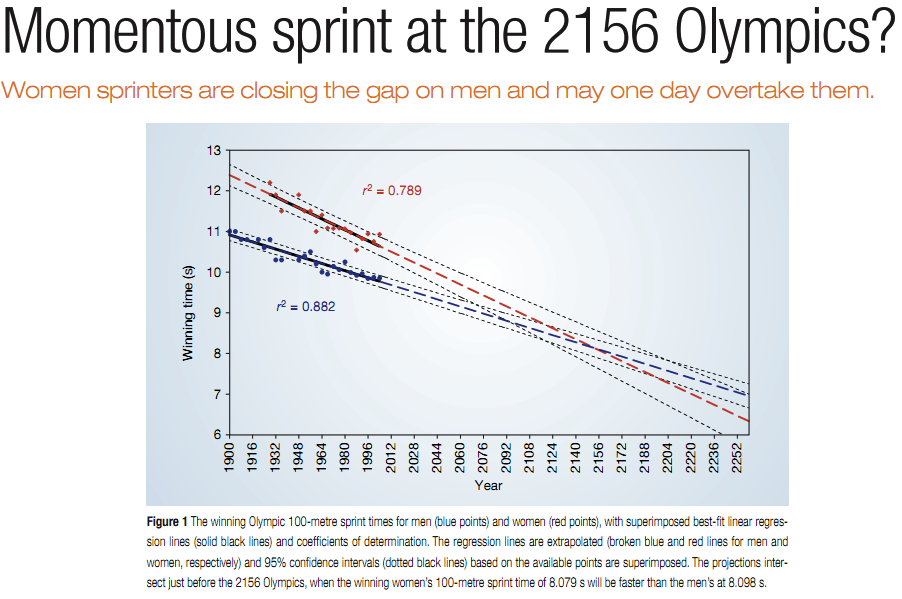
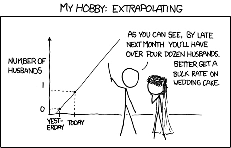
Applying a model estimate to values outside of the realm of the original data is called extrapolation.
Sometimes the intercept might be an extrapolation.
Examples of extrapolation
Examples of extrapolation
Examples of extrapolation1
To Come
We now have our first statistical model. In the coming lectures, we will talk about what this model means, how we use it, and how we can determine uncertainty in the model (since it is statistical, after all!).