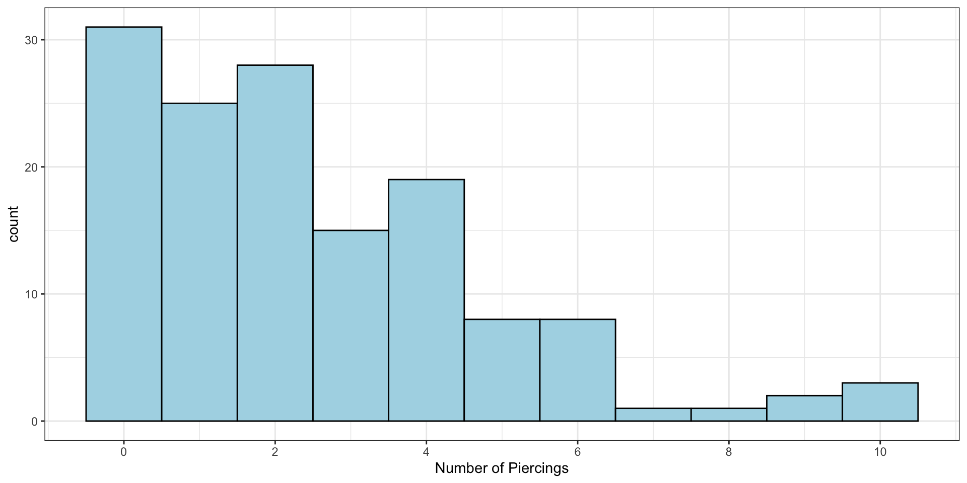
We can calculate the mean, variance, and standard deviation
piercings |>pull(`How many piercings do you have?`) |>mean()
[1] 2.503546
piercings |>pull(`How many piercings do you have?`) |>var()
[1] 5.39463
piercings |>pull(`How many piercings do you have?`) |>sd()
[1] 2.322634
The “average” student has 2.5 piercings…
Another Measure of Centre: Median
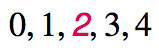
The median is the value that splits the data in half when ordered in ascending order.
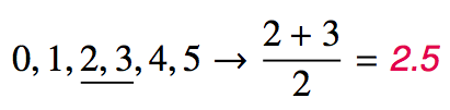
If there are an even number of observations, then the median is the average of the two values in the middle.
Since the median is the midpoint of the data, 50% of the values are below it. Hence, it is also the 50th percentile.
Calculating
Medians can’t really be computed with calculators, but we’ll use R for this anyway …
x <-c(1, 3, 8, 14, 21)median(x)
[1] 8
For our piercing data:
piercings |>pull(`How many piercings do you have?`) |>median()
[1] 2
The median, 2, is the number that splits the class in half – 50% have two or fewer piercings and 50% have two or more
Percentile
A percentile is the the smallest value from an ordered list of numbers which is greater than or equal to that percentage of list elements.
Example: The \(42^\text{nd}\) percentile of the numbers \(\{0, 1, 2, 3, \cdots, 99, 100 \}\) is 42.
It can become quite complicated when there aren’t an even multiple of 100 (and then + 1) items! (i.e., \(n \times 100 + 1\) items)
There are a few ways to calculate percentiles. As a result, we will use R exclusively for this.
Note
The 0 in the example is needed to make the quantile calculations “work”. If you were to try: quantile(0:100, probs = 0.42)
then you would get 42 as the result.
Special Names: Q1, Q3 and IQR
The 25th percentile is also called the first quartile, Q1.
The 50th percentile is also called the median.
The 75th percentile is also called the third quartile, Q3.
Between Q1 and Q3 is the middle 50% of the data. The range these data span is called the interquartile range, or the IQR.
\[
\text{IQR} = \text{Q3} - \text{Q1}
\]
Our Piercing Data : Median
0
0
0
0
0
0
0
0
0
0
0
0
0
0
0
0
0
0
0
0
0
0
0
0
0
0
0
0
0
0
0
1
1
1
1
1
1
1
1
1
1
1
1
1
1
1
1
1
1
1
1
1
1
1
1
1
2
2
2
2
2
2
2
2
2
2
2
2
2
2
2
2
2
2
2
2
2
2
2
2
2
2
2
2
3
3
3
3
3
3
3
3
3
3
3
3
3
3
3
4
4
4
4
4
4
4
4
4
4
4
4
4
4
4
4
4
4
4
5
5
5
5
5
5
5
5
6
6
6
6
6
6
6
6
7
8
9
9
10
10
10
NA
NA
NA
NA
NA
NA
NA
NA
NA
First 70 Ordered Observations
Median
Last 70 Ordered Observations
Our Piercing Data : Quartiles
0
0
0
0
0
0
0
0
0
0
0
0
0
0
0
0
0
0
0
0
0
0
0
0
0
0
0
0
0
0
0
1
1
1
1
1
1
1
1
1
1
1
1
1
1
1
1
1
1
1
1
1
1
1
1
1
2
2
2
2
2
2
2
2
2
2
2
2
2
2
2
2
2
2
2
2
2
2
2
2
2
2
2
2
3
3
3
3
3
3
3
3
3
3
3
3
3
3
3
4
4
4
4
4
4
4
4
4
4
4
4
4
4
4
4
4
4
4
5
5
5
5
5
5
5
5
6
6
6
6
6
6
6
6
7
8
9
9
10
10
10
NA
NA
NA
NA
NA
NA
NA
NA
NA
First Quarter
Third Quarter
Second Quarter
Fourth Quarter
Calculating
Quantiles are actually hard to do with calculators, but R makes it easy.
x <-sample(1:100, size =20, replace =TRUE)quantile(x, probs =c(0.4, 0.6))
 40%  60%
40.6 51.8
This computes the 40th and 60th percentiles of the vector, x, created by randomly sampling the values from 1 to 100 with replacement.
We introduced histograms earlier as our first numerical summary plot. Let’s see what else people have developed as tools for visualizing and exploring data.
Box Plot
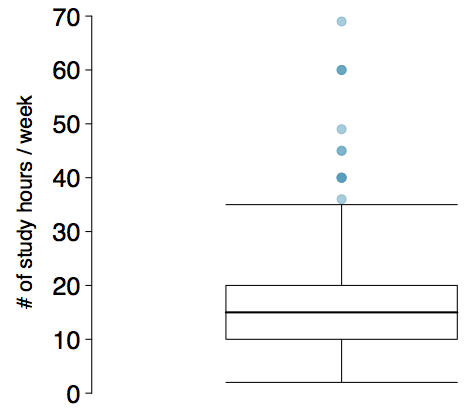
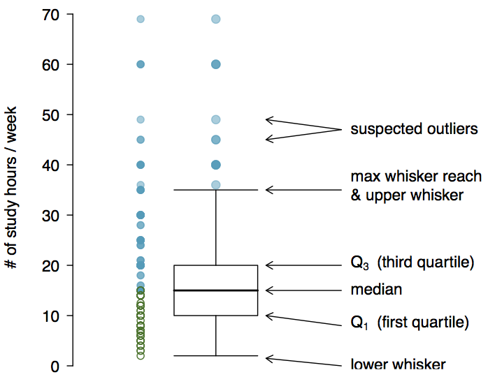
Box plots were developed by John Tukey in 1970, and popularized in his book Exploratory Data Analysis in 1977. The box in a box plot represents the middle 50% of the data, and the thick line in the box is the median.
Anatomy of a Box Plot
Piercing Boxplot
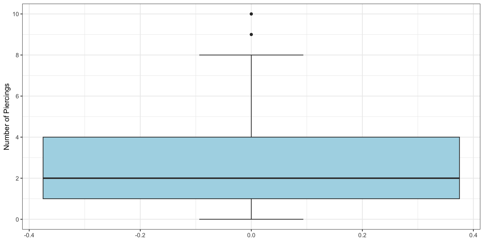
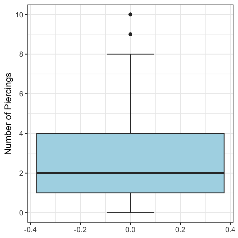
Let’s make a boxplot for our piercing example:
Min: 0
Q1: 1
Q2: 2
Q3: 4
Max: 10
Whiskers and Outliers
The whiskers of a box plot can extend up to \(1.5 \times \text{IQR}\) away from the quartiles.
max upper whisker reach = \(\text{Q3} + 1.5 \times \text{IQR}\)
max lower whisker reach = \(\text{Q1} - 1.5 \times \text{IQR}\)
A potential outlier is defined as an observation beyond the maximum reach of the whiskers. It is an observation that appears extreme relative to the rest of the data.
Whisker Notes
The whiskers, in general, will not be at \(\text{Q3} + 1.5 \times \text{IQR}\) and \(\text{Q1} - 1.5 \times \text{IQR}\)
These are merely the largest and smallest possible values.
The whisker stops at the smallest and largest values within 1.5 IQR of the quartiles.
For our dataset, that’s 0 and 8.
Outliers (continued)
Why is it important to look for outliers?
Identify extreme skew in the distribution.
Identify data collection and entry errors.
Provide insight into interesting features of the data.
Important
Skew is something we are going to be checking once we start statistical inference later in the course.
Robust Statistics
Median and IQR are more robust to skewness and outliers than mean and SD. Therefore,
for skewed distributions it is often more helpful to use median and IQR to describe the center and spread
for symmetric distributions it is often more helpful to use the mean and SD to describe the centre and spread
If you would like to estimate the typical household income for a student, would you be more interested in the mean or median income?
Robust Statistics
Median and IQR are more robust to skewness and outliers than mean and SD. Therefore,
for skewed distributions it is often more helpful to use median and IQR to describe the centre and spread
for symmetric distributions it is often more helpful to use the mean and SD to describe the centre and spread
If you would like to estimate the typical household income for a student, would you be more interested in the mean or median income?
Median
Mean versus Median
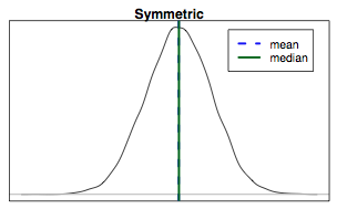
If the distribution is symmetric, centre is often defined as the mean:
mean \(\approx\) median
Mean versus Median
If the distribution is skewed or has extreme outliers, centre is often defined as the median
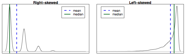
Right-skewed: mean > median
Left-skewed: mean < median
Practice
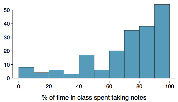
Which is most likely true for the distribution of percentage of time actually spent taking notes in class versus browsing your favourite social media feed?
mean > median 3. mean \(\approx\) median
mean < median 4. impossible to tell
Practice
Which is most likely true for the distribution of percentage of time actually spent taking notes in class versus browsing your favourite social media feed?
If we compute, the mean = 76% and the median = 80%. So …
mean > median 3. mean \(\approx\) median
mean < median 4. impossible to tell
Scatterplots
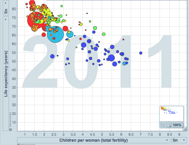
Scatterplots are useful for visualizing the relationship between two numerical variables. They will be incredibly important and we will spend a lot of time making them, and analyzing them.
Do life expectancy and total fertility appear to be associated or independent?
They appear to be linearly and negatively associated: as fertility increases, life expectancy decreases.
Was the relationship the same throughout the years, or did it change?
A table that summarizes data for two categorical variables is called a contingency table.
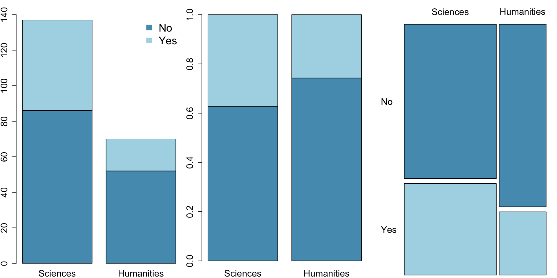
The contingency table below shows the distribution of students’ degree programs and whether or not they are looking for a life partner while in university.
Looking for Life Partner
No
Yes
Total
Program
Sciences
86
51
137
Humanities
52
18
70
Total
138
69
207
Bar Plots
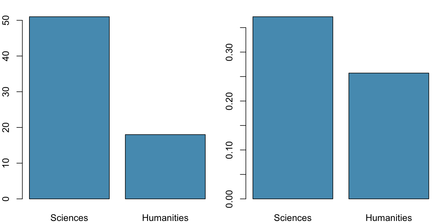
A bar plot is a common way to display a single categorical variable. A bar plot where proportions instead of frequencies are shown is called a relative frequency bar plot.
How are bar plots different than histograms?
Bar plots are used for displaying distributions of categorical variables
The height of each bar represents the number of observations in each category,
Histograms are used to display the distributions of numerical variables.
The height of each bar represents the number of observations in each interval (or bin).
The \(x\)-axis in a histogram is a number line, hence the order of the bars cannot be changed, while in a bar plot, the categories can be listed in any order
some orderings make more sense than others, especially for ordinal variables (shocking, I know :) )
The Main Point
Both bar plots and histograms are counting the number of observations.
However, bar plots are for categorical data, and histograms are for numerical data.
Choosing the Appropriate Proportion
Does there appear to be a relationship between a student’s major and whether the student is looking for a life partner in university?
Looking for Life Partner
No
Yes
Total
Major
Sciences
86
51
137
Humanities
52
18
70
Total
138
69
207
To answer this question we examine the row proportions:
% Science majors looking for a life partner: 51 / 137 ~ 0.37
% Humanities majors looking for a life partner: 18 / 70 ~ 0.26
Segmented Bar and Mosaic Plots
What are the differences between the three visualizations shown below?
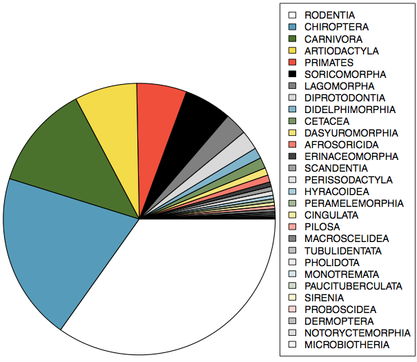
Pie Charts
Can you tell which order encompasses the lowest percentage of mammal species1?
Comparing Numerical Data Across Groups
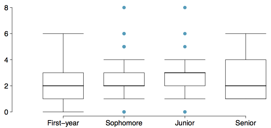
Does there appear to be a relationship between class year and the number of clubs students are in?
A Few Notes
Visualizing your data using an appropriate choice of plot is recommended as the first thing you do with a data set, regardless of your objective. The human eye is very, very good at seeing patterns and detecting things that do not belong.
However, if you use the wrong visualization, it can be either useless, or actively deceiving.
We will practice visualization-making in R during the Labs.