MATH 1051 - Lecture 03

Examining Scientific Papers & Numerical Variable Concepts

Kat Clark & Wesley Burr

Trent University

Today’s Topics

• Actual scientific experiments, available to you on Blackboard.
• Describing data
  • intro to parameters vs. statistics
• Plotting data
  • the idea of the histogram
  • modality
  • skewness
• Measures of centre
  • mean
• Measures of spread
  • variance, standard deviation

Readings

• Referenced scientific papers
• Chapters 5-6 in Introduction to Modern Statistics (2e).

Experiments and Observational Studies

Study 1

Maths anxiety in primary and secondary school students: Gender differences, developmental changes and anxiety specificity

Hill, Mammarella, Devine, Caviola, Passolunghi and Szűcs (2015)

(plain text abstract on next slide)

Study 1: Abstract

Maths anxiety (MA) is a debilitating negative emotional reaction towards mathematics. However, MA research in primary and early secondary school is surprisingly sparse and inconsistent. Here we tested primary and secondary students’ maths and reading performance and their maths and general anxiety (GA). We examined gender differences, developmental changes regarding the MA/maths performance link and investigated whether MA is linked to other academic domains (reading) and/or to other anxiety-types (GA). Results revealed that girls exhibited higher MA than boys at both educational levels. Whilst there was a reliable negative correlation between MA and secondary students’ arithmetic performance, no such relationship was revealed in primary students. Finally, MA was moderately correlated with GA and, when GA was partialled out, MA remained significantly correlated with secondary students’ arithmetic performance. MA was not related to reading performance when GA was controlled. It was concluded that the negative MA/maths performance link surfaces later in the educational timeline and MA appears to be both exclusively related to maths and independent of GA.

Study 1

What can we say about this study?

• primary and secondary students, maths, reading, general anxiety
• exhibited, reliable negative correlation
• relationship
• moderately correlated
• exclusively related

Experiment or observational study? 📊

Do we know what kind of study it is?

Experiment or observational study?

• The cohort consisted of 1014 children attending both primary and secondary schools in Italy. We excluded some children due to missing data, so the final sample consisted of 981 students …
• The Abbreviated Math Anxiety Scale is a self-report MA questionnaire. Using a 5-point Likert scale, participants indicate how anxious (e.g. 1 = low anxiety; 5 = high anxiety) they would feel during certain situations involving maths.
• Researchers administered the tests in school.
• Children were tested in the classroom in group sessions each lasting approximately 1 h.
• Materials were administered in a fixed order: arithmetic test, reading comprehension test, RCMAS-2 and AMAS. The questionnaires were administered last in order to avoid stereotype threat effects.

More Details

• Although our results suggest that the negative relationship between MA and maths performance may not develop in primary school, MA was still present at this age and primary students may not possess the coping strategies or cognitive maturity to deal effectively with their maths-related worries.
• Additionally, our findings suggest that a negative link between MA and maths performance is likely to develop as students are faced with increasing educational demands in secondary school.
• Our findings thus highlight the need to:
  1. provide more emotional support to primary students suffering from MA and;
  2. develop preventative, protective measures aimed at halting the emergence of MA in primary school in order to reduce effects on performance in secondary education

Study 2

Sex Differences in Dieting Trends, Eating Habits, and Nutrition Beliefs of a Group of Midwestern College Students

Davy, Benes and Driskell (2006)

(plain text abstract on next slide)

Study 2: Abstract

The influence of sex on dietary trends, eating habits, and nutrition self-assessment and beliefs of a group of college students at a large Midwestern university was investigated. A questionnaire was completed by 105 male and 181 female undergraduate students. Men had significantly higher (P<0.0001) height, weight, and body mass index values. Significantly higher percentages of women than men had tried a low-fat diet (P=0.0075) and a low-carbohydrate diet (P=0.0285). Significantly lower percentages of women than men had never tried a diet (P=0.0173). Significantly higher percentages of women than men reported gaining nutrition knowledge from family (P=0.0033) and magazines/newspapers (P=0.0345). […]

Study 2: Abstract (Continued)

[…] Significantly higher percentages of women than men agreed that they had too much sugar in their diets (P=0.0157), that it is important to limit carbohydrate consumption (P=0.0077), that it is important to limit the amount of fat consumed to lose weight (P=0.0194), and that they needed to lose weight (P<0.0001). It is important to eat a variety of foods for good health according to 94.4% of subjects. Sex differences existed in these college students with regard to anthropometric measurements, certain choices of diets, some sources of nutrition knowledge, and some nutrition beliefs.

Study 2

What can we say about this study?

• questionnaire
• 105 male, 181 female
• comparing men to women
• lots of “P” things?

Experiment or observational study? 📊

Do we know what kind of study it is?

Experiment or observational study?

• A 21-item questionnaire was developed that assessed self-reported anthropometric measurements, use of specific diets … the questionnaire was pilot-tested with 10 undergraduate students to clarify language and response options. Eleven students completed the questionnaire again after 4.5 weeks; responses were the same 78% of the time.
• Participants were recruited from an introductory nutrition course during the fourth week of the 2005 spring semester; 100% of eligible students participated and all signed informed consent forms.
• Each subject’s classification and college was obtained from class rosters and compared with that of the university’s undergraduate population (17).

More Details

• Several sex differences in anthropometric measurements and certain choices of diets, sources of nutritional knowledge, and nutrition were observed in a group of college students.
• These college men and women seemingly related to some nutrition issues differently.
• Registered dietitians and other health professionals should take these differences into account when developing nutrition education materials and designing nutrition intervention programs for college students and other young adults.

Study 3

Early life history transitions and recruitment of Picea mariana in thawed boreal permafrost peatlands

Camill, Chihara, Adams, Andreassi, Barry, Kalim, Limmer, Mandell and Rafert (2010)

(plain text abstract on next slide)

Study 3: Abstract

Black spruce (Picea mariana) is the most abundant tree species in the boreal biome, but little is known about how climate warming may change recruitment in peatlands, especially those affected by permafrost thaw. We used results from a seven-year study in northern Manitoba, Canada, to address the following questions: (1) What is the relative importance of early life history transitions on P. mariana recruitment? (2) How are these transitions mediated by biological and environmental factors, including competition, facilitation, disease, herbivory, water table depth, and soil nutrients? (3) Do interactions among these factors create additional recruitment limitations beyond those imposed by environmental factors changing with climate warming, such as hydrology? Seed rain was measured over six years on forested permafrost plateaus and in neighboring collapse scar bogs. Seed germination and seedling survival and growth were measured over 4–5 years in collapse scars and assessed across a three-level water table treatment. […]

Study 3: Abstract (Continued)

[…] Survival and growth experiments examined additional combinations of above- and belowground vascular plant competition and fertilizer addition. Results showed that failure of germination and survival on growing moss surfaces and reduced survival of seedlings in wetter microsites were primary constraints. Seed influx was significantly lower in collapse scars but likely did not limit recruitment. Biological and environmental factors mediating these life history transitions also differed in relative importance, and interactions among them tended to amplify recruitment limitation. Seedling survival was most strongly controlled by fast-growing mosses in wet microsites but also was influenced by apparent drowning in wet plots, herbivory, and loss of foliage caused by a fungal pathogen. Seedling growth was strongly controlled by water table depth, nutrient and competition levels, and fungal pathogens. Multiple, interacting factors will affect P. mariana establishment in boreal peatlands during climate warming. Generalizations about recruitment relying on few environmental gradients sensitive to climate change, such as water table, may therefore not fully capture the complexities of establishment.

Study 3

What can we say about this study?

• 7 year study
• Manitoba, Canada
• studying black spruce (Picea mariana)
• climate warming, permafrost
• “recruitment” in peatlands

Experiment or observational study? 📊

Do we know what kind of study it is?

Experiment or observational study?

• Seed germination and seedling survival and growth were measured over 4–5 years in collapse scars and assessed across a three-level water table treatment.
• Survival and growth experiments examined additional combinations of above- and belowground vascular plant competition and fertilizer addition

More Details (from the paper)

• Seed rain was measured over six years (1997–2002) using traps located randomly on permafrost plateaus and neighboring collapse scars to quantify P. mariana fecundity on plateaus and dispersal into neighboring collapse scars.
• Stand densities on plateaus ranged from 5000–8000 trees per hectare in this region (Camill 1999a, Camill et al. 2001). Seed traps were 0.17 m 2 polypropyl- ene boxes lined with fiberglass mesh.
• Traps were placed in three replicate plateau/scar sites (Fig. 1B) in each of four study zones for a total of 12 sites in the seed rain analysis. Each site contained 10 plateau traps and five scar traps for the first two years (1997–1998), but the number of collapse scar traps per site was increased to 15 from 1999 to 2002 for better spatial coverage and sampling intensity.

More Details

Germination, growth and survival experiments

• Seed germination and seedling survival and growth in thawed collapse scars were measured over 4–5 years following experimental additions of seeds and seedlings in a single peatland landscape (Fig. 1C).
• located 15 collapse scar sites separated by distances of 100 m to 5 km.
• We stratified each site into three water table depth categories, corresponding to the dominance of three Sphagnum species: wet, medium, and dry
• Thirty plots were located in each of the wet, medium, and dry water table microhabitats for a total of 90 plots in the 15 collapse scar sites.
• We placed multiple plots in larger collapse scar sites to constrain random variability, but to avoid pseudoreplication, we averaged data from multiple plots per water table treatment to generate a single mean per site, and we handled site, water table categories, and plot treatments as random effects in statistical analysis (see Methods: Statistical analyses).

More Details

• We also measured P. mariana seedling survival and growth over a five-year period by transplanting 2160 one-year-old, containerized nursery seedlings grown from seed collected within 80 km from the study site (Tolko Industries, The Pas, Manitoba and Pineland Nurseries, Hadashville, Manitoba, Canada).
• A randomized \(3\times 2\times 2\) split–split plot design was established by first stratifying plots across three levels of water table depth, then subdividing each plot into four subplots randomly assigned to all combinations of a two-level nutrient amendment treatment (fertilized/unfertilized) and a two-level above- and belowground vascular plant competition experiment (competition removed/competition present).

Conclusion

1. This was definitely an experiment
2. Randomization was used
3. Stratification was applied on the sites
4. Something called a “split-split plot design” was used
5. Treatments mentioned - nutrient amendment, above- and below-ground plant competition, and water level

No blinding, blocking, or placebo - this wasn’t a study on people, and blocking wasn’t required (although stratification produced an additional treatment variable, which was of interest)

Study 4

Supplemental Perioperative Oxygen To Reduce The Incidence of Surgical-Wound Infection

Greif, Akca Horn, Kurz, Sessler, for the Outcomes Research Group (2000)

Study 4: Abstract

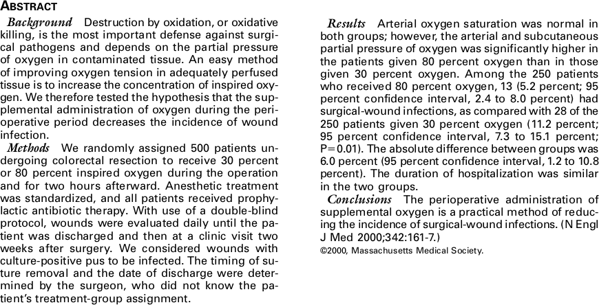
Background: Destruction by oxidation, or oxidative killing, is the most important defense against surgical pathogens and depends on the partial pressure of oxygen in contaminated tissue. An easy method of improving oxygen tension in adequately perfused tissue is to increase the concentration of inspired oxygen. We therefore tested the hypothesis that the supplemental administration of oxygen during the perioperative period decreases the incidence of wound infection.

Methods: We randomly assigned 500 patients undergoing colorectal resection to receive 30 percent or 80 percent inspired oxygen during the operation and for two hours afterward. Anesthetic treatment was standardized, and all patients received prophylactic antibiotic therapy. With use of a double-blind protocol, wounds were evaluated daily until the patient was discharged and then at a clinic visit two weeks after surgery. We considered wounds with culture-positive pus to be infected. The timing of suture removal and the date of discharge were determined by the surgeon, who did not know the patient’s treatment-group assignment. […]

Study 4: Abstract (Continued)

[…]

Results: Arterial oxygen saturation was normal in both groups; however, the arterial and subcutaneous partial pressure of oxygen was significantly higher in the patients given 80 percent oxygen than in those given 30 percent oxygen. Among the 250 patients who received 80 percent oxygen, 13 (5.2 percent; 95 percent confidence interval, 2.4 to 8.0 percent) had surgical-wound infections, as compared with 28 of the 250 patients given 30 percent oxygen (11.2 percent; 95 percent confidence interval, 7.3 to 15.1 percent; P=0.01). The absolute difference between groups was 6.0 percent (95 percent confidence interval, 1.2 to 10.8 percent). The duration of hospitalization was similar in the two groups.

Conclusions: The perioperative administration of supplemental oxygen is a practical method of reducing the incidence of surgical-wound infections. (N Engl J Med 2000;342:161-7.)

Study 4

What can we say about this study?

• random assignment of 500 patients
• 30% or 80% inspired oxygen
• double-blind protocol
• some stats-y sounding stuff

Experiment or observational study? 📊

Do we know what kind of study it is?

Experiment or observational study?

• After the induction of anesthesia and endotracheal intubation, each patient was assigned to one of two groups through the use of a set of computer-generated random numbers.
• The assignments were stratified according to the participating hospital and were kept in sealed, sequentially numbered envelopes until used.
• One group of patients received 30 percent oxygen and 70 percent nitrogen; the other group received 80 percent oxygen and 20 percent nitrogen.

More Details

• The anesthesiologists who cared for the patients were aware of their treatment-group assignments.
• However, cardboard shields were positioned over flowmeters and relevant monitors to prevent the surgical team from determining the fraction of inspired oxygen.
• Two hours after a patient’s recovery from anesthesia, the record of the administration of anesthesia and the blood gas results were sealed so that the surgeons and investigators who evaluated the wounds post-operatively would be unaware of the patients’ treatment-group assignments.
• Patients were not informed of their group assignments.

More Details

From July 1996 to October 1998, we enrolled 500 patients:

• 223 (45 percent) at the Donauspital (Vienna, Austria),
• 213 (43 percent) at the University of Vienna (Vienna, Austria), and
• 64 (13 percent) at the University Hospital Eppendorf (Hamburg, Germany).

Enrollment in the study was discontinued after 500 patients had been enrolled because the incidence of surgical-wound infection in the two groups differed significantly (P<0.012).

More Details

• In summary, the administration of supplemental oxygen during colorectal resection and for two hours afterward halved the incidence of surgical-wound infection.
• Because the cost of and risk associated with supplemental perioperative oxygen are trivial, the provision of supplemental oxygen appears to be a practical method of reducing the incidence of this dangerous and expensive complication.

Some Key Take-Aways

Language

• If a paper uses the language of “correlated” and “associated” and “relationships”, it’s probably an observational study, even if you know nothing else about it.
  • If researchers can use causal language, they will.
• If a paper says “caused” or “implies”, it’s probably an experiment, although sometimes this sneaks through - this isn’t 100%.

Methods

• If the paper involves a questionnaire, it’s almost certainly an observational study.
• If the words “randomized” or “randomly” appear in the methods, that’s a good sign (recall the diagram!).
• If blinding, blocking, or stratification appear, that’s also a good sign that you might be looking at an experiment.

At the end of the day …

• The real key is to look for treatments.
• If you see the experimenters doing something which changes their experimental units or materials, that’s an experiment.
• If there’s randomization, it’s a random experiment. Surveys are just observations.

Examining Numerical Data

Numerical Data

• If we have numerical data, as discussed previously, we have one or more variables which is numeric in type.
• This means, coarsely, that we can compute an average or a sum on the data, and it makes some kind of sense!
• But why do we gather and/or analyze numerical data?

Parameters vs. Statistics

• We’re almost always interested in some aspect of the population, often a population parameter, or just parameter for short.
• We could find the parameter if we sample the entire population (census).
• Normally, we have to estimate it from a sample using a sample statistic, or just statistic.

We will return to this idea over the course continuously! For now:

• a parameter represents some truth about the population; and
• a sample statistic is our best estimate of the parameter based on a sample.

Our First Statistic: The Mean

• The sample mean, denoted as \(\bar{x}\), can be calculated as \[ \bar{x} = \frac{x_1 + x_2 + \cdots + x_n}{n} = \frac{1}{n} \sum_{i=1}^{n} x_i \] where \(x_1, x_2, \cdots, x_n\) represent the \(n\) observed values.
• The population mean is also computed the same way but is denoted as \(\mu\). It is often not possible to calculate \(\mu\) since all of the population data are rarely available.
• The sample mean is a sample statistic, and serves as a point estimate of the population mean. This estimate may not be perfect, but if the sample is good (representative of the population), it is usually a pretty reliable estimate.

Calculating

We will never expect you to compute a mean without a calculator. In practice, we do this using R almost always. For example,

x <- c(1, 3, 8, 14, 21)
mean(x)

[1] 9.4

Visualizing Data

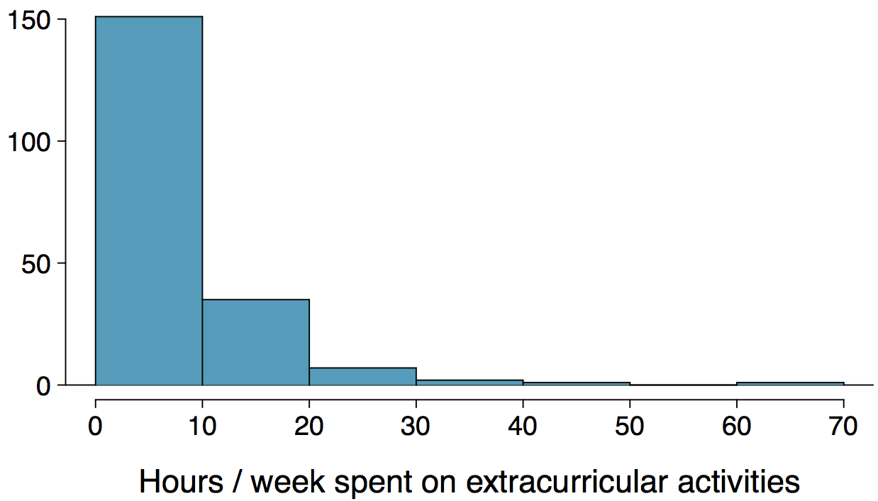
Histograms \(-\) Extracurricular Hours

• Histograms provide a view of data density for numerical data. Higher bars represent where the data are relatively more common.
• Histograms are especially convenient for describing the shape of the data distribution, as well as the modality
• The chosen bin width can alter the story the histogram is telling¹.

1. https://tinlizzie.org/histograms/

Bin Width

Which one(s) of these histograms are useful? Which reveal too much about the data? Which hide too much? 📊

Shape of a Distribution: Modality

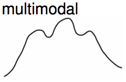
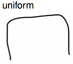
Does the histogram have a single prominent peak (unimodal), several prominent peaks (bimodal/multimodal), or no apparent peaks (uniform)?

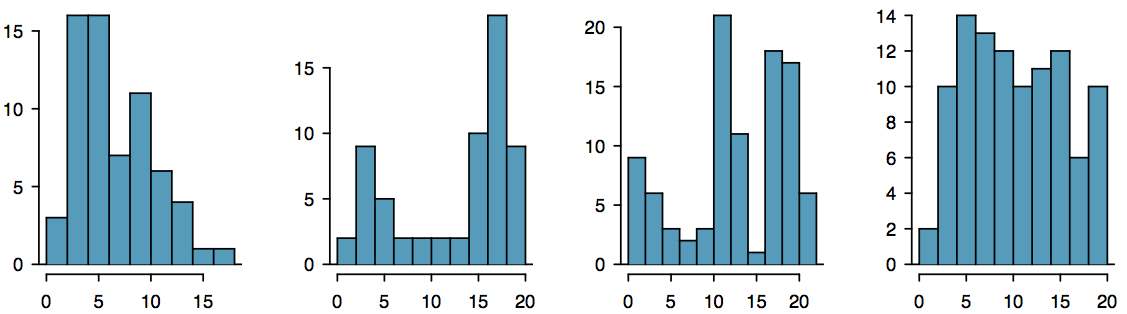
Note: In order to determine modality, step back and imagine a smooth curve over the histogram – imagine that the bars are wooden blocks and you drop a limp spaghetti over them, the shape the spaghetti would take could be viewed as a smooth curve.

Shape of a Distribution: Skewness

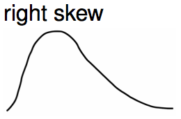
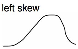
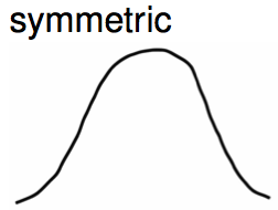
Is the histogram right skewed, left skewed or symmetric?

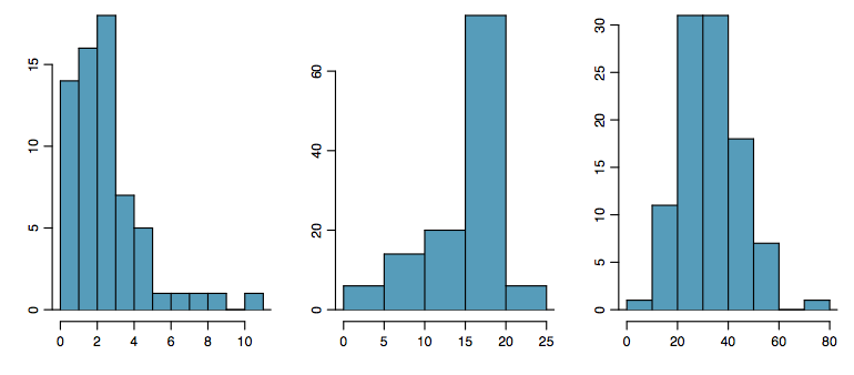
Histograms are said to be skewed to the side of the long tail.

Shape of a Distribution: Unusual Observations

Are there any unusual observations or potential outliers?

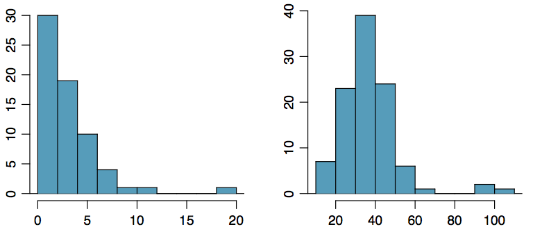
Commonly observed shapes of distributions

Modality

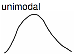
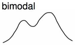
Skewness

Practice

Which of these variables do you expect to be uniformly distributed? 📊

1. weights of adult rhinos
2. salaries of a random sample of people from North Carolina
3. house prices
4. birthdays of classmates (day of the month)

Practice

Which of these variables do you expect to be uniformly distributed?

1. weights of adult rhinos
2. salaries of a random sample of people from North Carolina
3. house prices
4. birthdays of classmates (day of the month)

Application Activity: Shapes of Distributions

Sketch the expected distributions of the following variables:

• number of piercings per person 📊
• scores on an exam in percentages
• IQ scores

Come up with a concise way (1-2 sentences) to teach someone how to determine the expected distribution of any variable.

Are you typical?

How useful are centres alone for conveying the true characteristics of a distribution?

NPR’s Planet Money did an episode on the “modal American”¹.

1. https://www.npr.org/2019/08/28/755191639/episode-936-the-modal-american

Average American

This is an example from the podcast:

One of the individuals being interviewed had seen a tweet going around about average income in the US:

“But it was like - they had - I don’t know - $60,000 in labor income and $10,000 in Social Security income. I’m like, well, OK. Now hold on a second. No, they don’t. That’s not a person.”

“You are probably working or you’re collecting Social Security and almost certainly not both.”

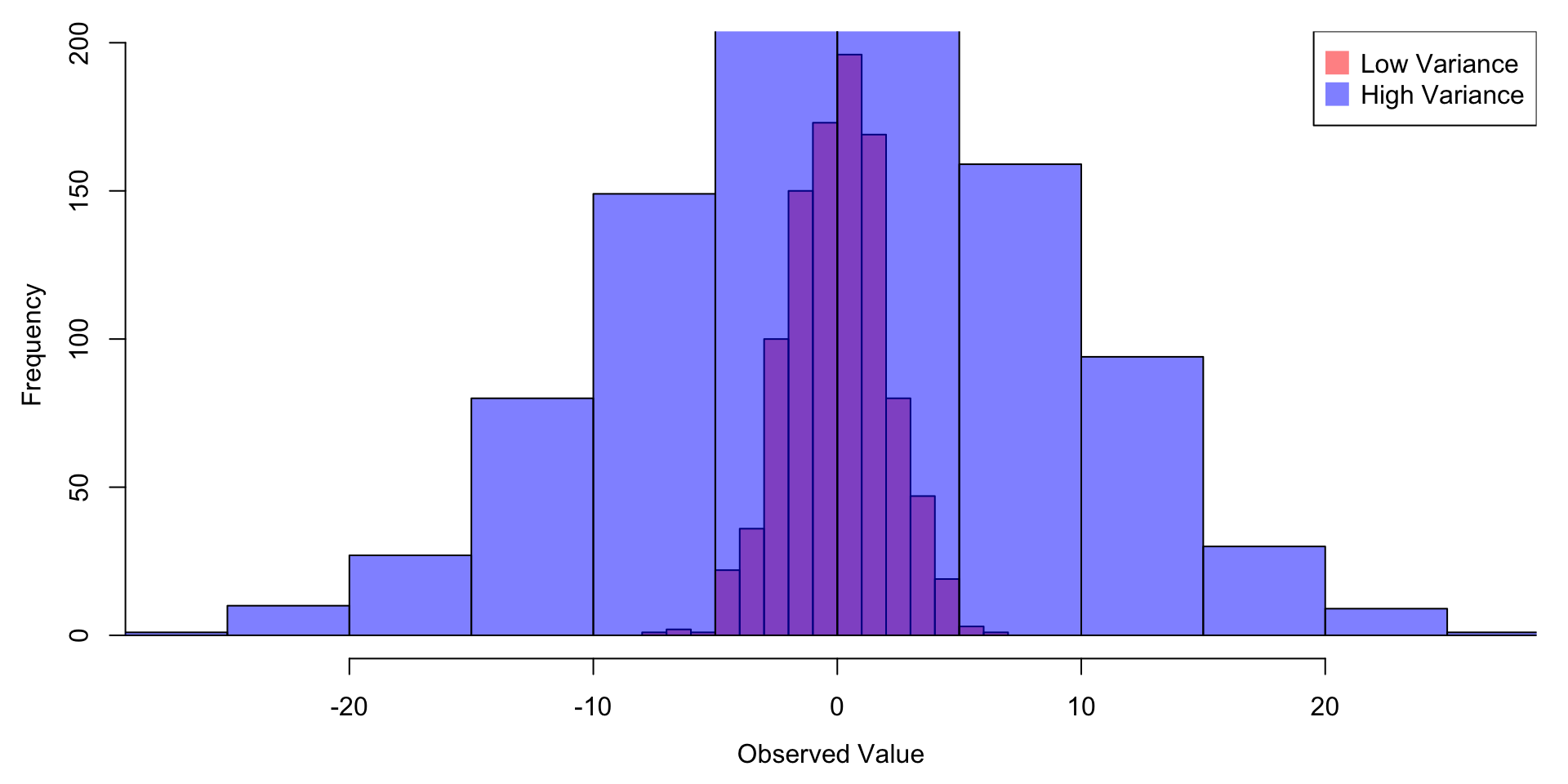
Another Way of Summarizing: Variance

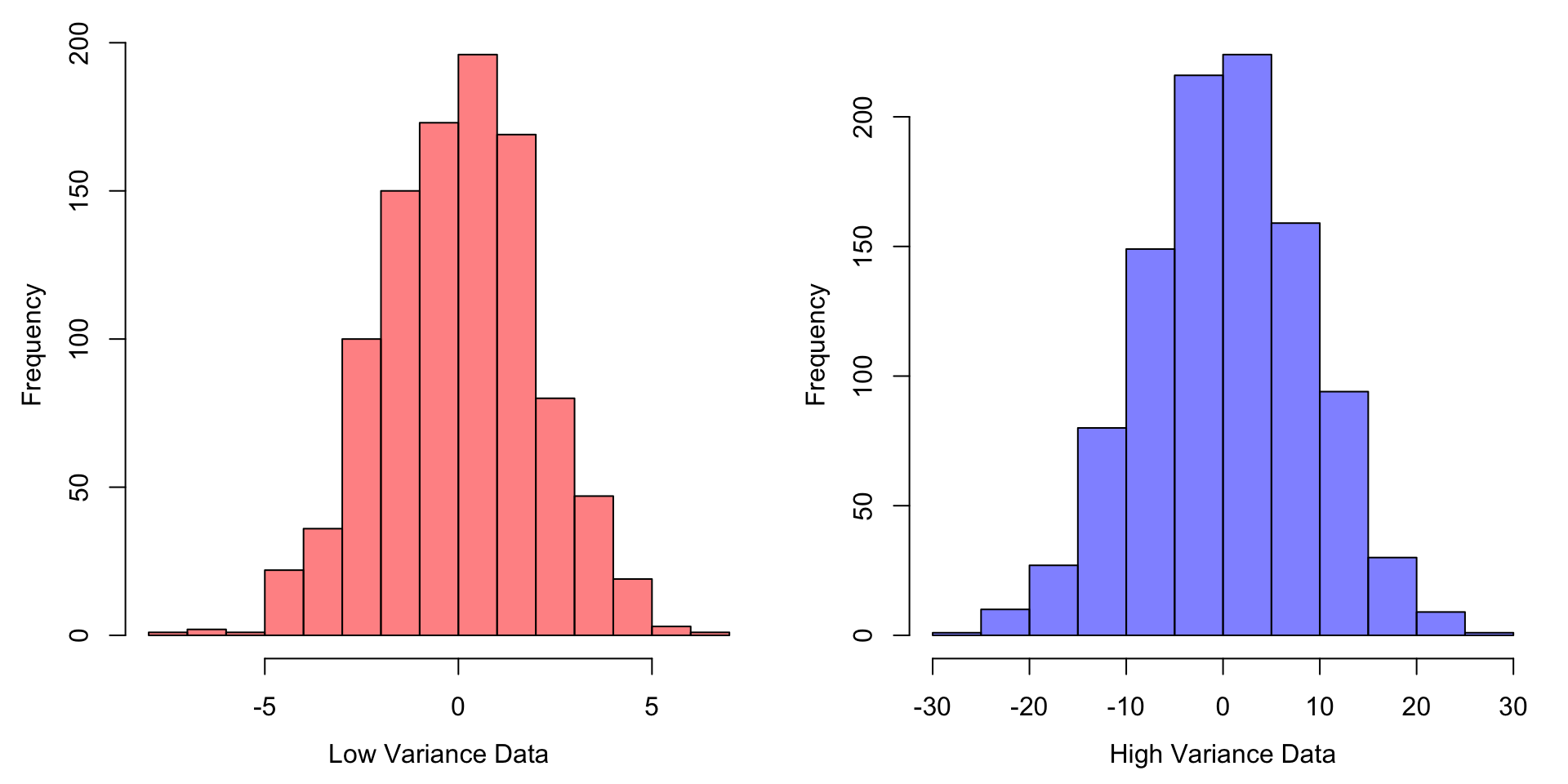
Variance describes the spread of the data.
The units of the variance are the square of the data’s units¹.

1. This is because of how variance in calculated; shown on the next slide!

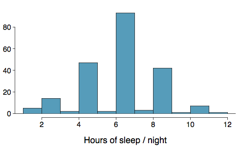
Variance

Variance is roughly the “mean of the squared deviation from the mean”.

\[ s^2 = \frac{1}{n-1} \sum_{i=1}^{n} (x_i - \bar{x})^2 \]

• The sample mean is \(\bar{x} = 6.71\), and the sample size is \(n = 217\).
• The variance of the amount of sleep students get per night can be calculated as:

\[ \begin{split} s^2 &= \frac{1}{217 - 1} \left[ (5-6.71)^2 + (9-6.71)^2 + \cdots + (7-6.71)^2 \right] \\ &= 4.11 \text{ hours}^2 \end{split} \]

Variance (continued)

Why do we use the squared deviation in the calculation of variance?

• To get rid of negatives so that observations equally distant from the mean are weighted equally.
  • We want to know how far from the mean an observation is; the direction doesn’t matter.
• To weight larger deviations more heavily.
  • If an observation is two times as far away from the mean as another observation, then it contributes four times as much to the sum!

Standard Deviation

The standard deviation is the square root of the variance, and has the same units as the data.

\[ s = \sqrt{s^2} \]

The standard deviation of the amount of sleep students get per night can be calculated as: \[ s = \sqrt{4.11} = 2.03 \text{ hours} \]

Important

The concept of the standard deviation is something we will use A LOT!

Standard Deviation and Sleep Data

We can see that all of the data are within 3 standard deviations (\(s = 2.03\) hours) of the mean (\(\bar{x} = 6.17\)).

Calculating

We will never expect you to compute a variance or SD without a calculator. In practice, we do this using R almost always. For example,

x <- c(1, 3, 8, 14, 21)
var(x)

[1] 67.3

sd(x)

[1] 8.203658

sqrt(var(x))

[1] 8.203658

Large Variance \(\rightarrow\) More Spread

Large Variance \(\rightarrow\) More Spread