Lecture 06 - Trees

AMOD-5440

Kat Clark

Trent University

2026-10-16

Trees

Classification and Regression Trees

• Our next topic is the use of tree-based methods for regression and classification.
  • These methods often use the acronym CART, which stands for Classification and Regression Trees.
• Trees involve stratifying (or segmenting) the predictor space into a number of simple regions.
• In order to make a prediction for a given observation, we typically use the mean or the mode response value for the training observations in the region to which it belongs.
• Because the set of splitting rules used to segment the predictor space can be summarized in a tree, these types of approaches are known as decision tree methods.

Vocabulary

We describe trees using the following definitions:

• branch: result of a decision, departing a node, traveling either to another node or a leaf
• node: (or internal node): decision points, where branches fork
• leaf (also terminal node): final regions, on which estimates are created
• In computer science, trees are drawn upside down because the root is defined as the starting node, and by convention we draw hierarchies top-down so the flow from root to leaves is easy to follow.

Regression Trees

• Regression Trees are models, built on data just like we’ve been doing all along, where the predictors form a space.
• In that space, we divide the space into regions, and then predict the response on each sub-region.

Example - Baseball

Recall the example of Hitters¹ - the Major League Baseball example with characteristics of hitters in MLB in 1986, with their salaries being the response.

1. Lecture 4

Regression Trees: Simple Example

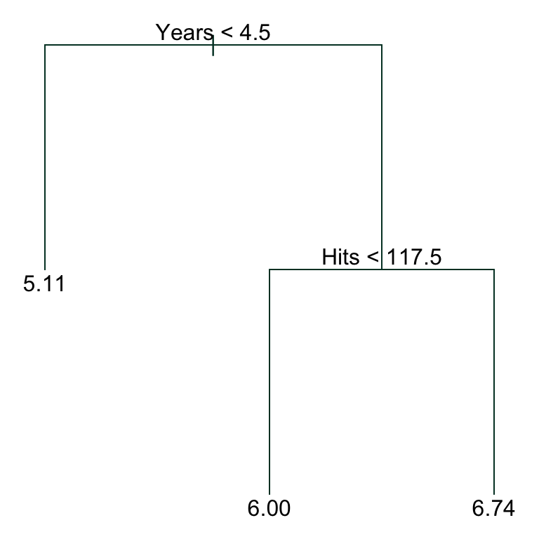
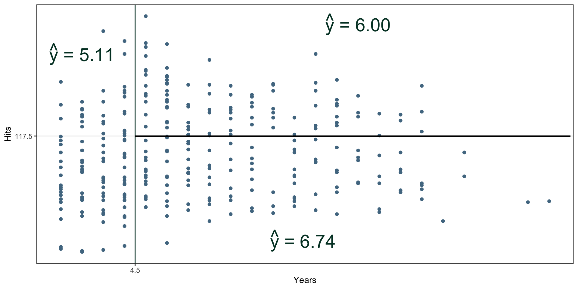
Consider the response variable \(\log(\)Salary\()\), and predictor variables Years and Hits.

• We divide on Years: less than 4.5 goes left, and more than 4.5 goes right
• The left branch then predicts a log-Salary of 5.11.
• The right branch splits further on whether the player had Hits last season < 117.5 or not; predicting 6.00 and 6.74 log-thousand dollar Salary, respectively.

Interpretation

• Years is the most important factor in determining Salary (hence being the primary - first - node), and players with less experience earn lower salaries than more experienced players.
• Given that a player is less experienced, the number of hits that he made in the previous year seems to play little role in his salary. But among players who have been in the major leagues for five or more years (right branch), the number of hits made in the previous year (node Hits < 117.5) does affect salary, and players who made more hits last year tend to have higher salaries.

How do Trees Actually Work?

Roughly speaking, two steps:

1. Divide the predictor space in \(J\) distinct, non-overlapping regions (a partition in mathematical terms), \(R_1, \cdots, R_J\).
2. For every observation in a given \(R_j\), compute the mean of the response values for observations in \(R_j\), make this the prediction.

Seems simple, right?

Ha. Haha.

• It turns out that step 1 is really tricky
• If we just considered every possible partition of the feature space, this is incredibly computational
• Instead, we do what is called recursive binary splitting - a greedy algorithm that splits one step at a time.

Greedy Splitting

The algorithm is called greedy because:

• at each step of the tree-building process, the best split is made for that step and only that step
  • there is no forward-looking aspect
  • think of mixed selection, which does “backward checks”.

So how does this work in practice?

1. Start by selecting the predictor \(X_j\) and cutpoint \(s\)
   • \(s\) is chosen such that splitting the predictor space into regions \(\{ X | X_j < s \}\) and \(\{ X | X_j \geq s \}\) results in the greatest possible reduction in RSS (Residual Sum of Squares).
   • Turns out, this isn’t too bad to compute.

Greedy Splitting

Next, we are greedy.

2. Pick one of the two regions we now have
   • look for the next best predictor whose splitting on a new cutpoint \(s\) will result in the greatest reduction in RSS.
   • this split is done, giving us three total regions.
3. Repeat this process, splitting one region at a time on each step, greedily reducing the most RSS possible at that step.

At some point, we have to stop, perhaps when no region contains more than some small number (e.g., 5) observations.

Example: Two Predictors

Overfitting

• Doing the previous process and separating the data into very small regions may produce good predictions on the training set, but is likely to massively overfit the data
  • the tree that results will likely be too complex to be flexible.
• The solution is to grow a very large tree, say \(T_0\), and then prune it back to obtain a subtree
  • however, using cross-validation on every possible subtree is computationally infeasible

Cost Complexity Pruning

Add a penalty, controlled by \(\alpha\), to the cost function for the tree, that is, \[ \sum_{m=1}^{|T|} \sum_{x_i \in R_m} (y_i - \hat{y}_{R_m})^2 + \alpha |T| \] so that we penalize having more nodes (\(|T|\)).

• The tuning parameter \(\alpha\) controls the trade-off between complexity and fit to the training data.
• When \(\alpha=0\), we just get the greedy overfit tree
  • as \(\alpha\) grows, we typically minimize the quantity above by having a smaller, less complex, tree

Choosing \(\alpha\)

• It turns out that obtaining a sequence of subtrees in this fashion is actually fairly simple, and we can then determine a value of \(\alpha\) using \(K\)-fold cross-validation or a validation (test) set.
  • This happens all the time in computer science (think binary search, quick sort, etc … )
• Once we have the \(\alpha\) chosen, return to the full data set / training set, and obtain the subtree corresponding to the use of \(\alpha\).

Summary

• Once you get your head around the idea of trees, with branches, leaves, and so on, the actual process of fitting the tree to the data is very similar to lasso
• We use the parameter \(\alpha\) (\(\lambda\)) to control the number of nodes (non-zero parameters) through penalization, using cross-validation to determine the value of the penalty.
• We then fit a model using the resulting parameter \(\alpha\) (\(\lambda\)) to the full training data set, create a prediction \(\hat{y}\), and evaluate it against some test set.

Trees versus Linear Models

Which model is better? It depends (a statistician’s favourite phrase!).

• If the relationship is well approximated by a linear structure, then regression will work well (as you would expect), and methods like regression trees that do not exploit the structure will not.
• However, if there are highly non-linear relationships between the response and predictors, decision trees may outperform.
• The relative performances can always be assessed by estimating the test error using CV or validation set approaches.

Advantages of Trees

• Trees are very easy to explain to people.
  • In fact, they are even easier to explain than linear regression!
• Some people believe that decision trees more closely mirror human decision-making than do the regression and classification approaches seen in previous chapters.
• Trees can be displayed graphically, and are easily interpreted even by a non-expert (especially if they are small).
• Trees can easily handle qualitative predictors without the need to create dummy variables.

Disadvantages of Trees

• Trees generally do not have the same level of predictive accuracy as some of the other regression and classification approaches seen in this book.
• Additionally, trees can be very non-robust. In other words, a small change in the data can cause a large change in the final estimated tree.

However, these disadvantages can be overcome by using methods like bagging, random forests and boosting; next, after an example.

Example: Boston Housing

set.seed(1)
boston_train <- sample(1:nrow(Boston), nrow(Boston)/2)
tree_boston <- tree(medv ~ ., Boston, subset = boston_train)
summary(tree_boston)

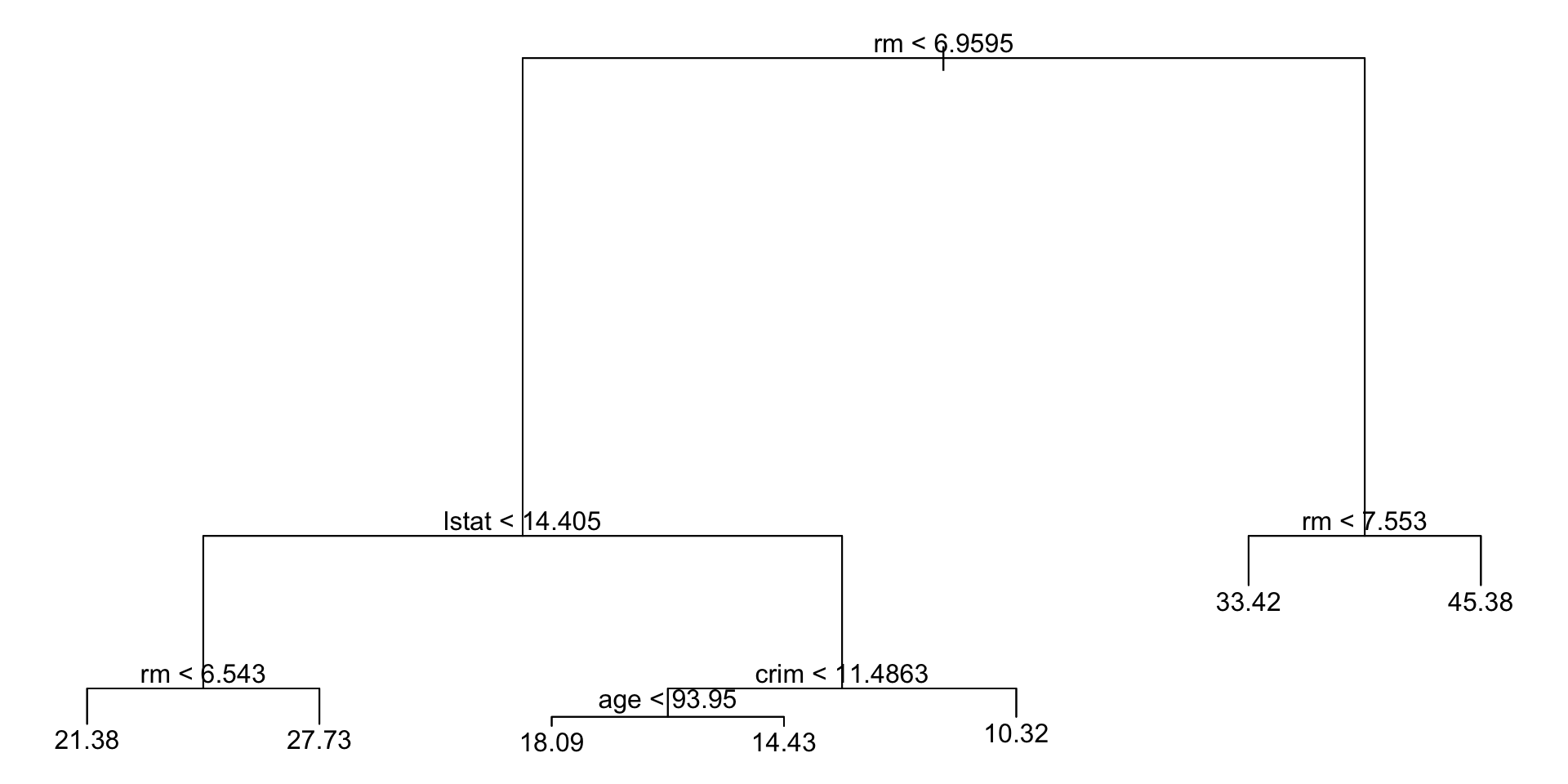
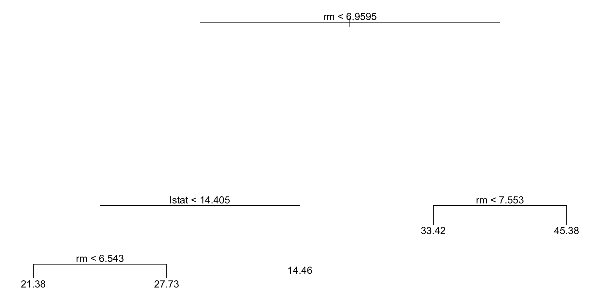
Regression tree:
tree(formula = medv ~ ., data = Boston, subset = boston_train)
Variables actually used in tree construction:
[1] "rm"    "lstat" "crim"  "age"  
Number of terminal nodes:  7 
Residual mean deviance:  10.38 = 2555 / 246 
Distribution of residuals:
    Min.  1st Qu.   Median     Mean  3rd Qu.     Max. 
-10.1800  -1.7770  -0.1775   0.0000   1.9230  16.5800 

Example: Boston Housing

par(mar = c(1,1,1,1))
plot(tree_boston)
text(tree_boston)

Example: Boston Housing

cv_boston <- cv.tree(tree_boston, K = 10)
ggplot(data = NULL, aes(x = cv_boston$size, y = cv_boston$dev)) +
  geom_point() + geom_line() + scale_x_continuous(breaks = 1:7) +
  labs(x = "# Terminal Nodes", y = "RSS") + theme_bw()

Example: Boston Housing

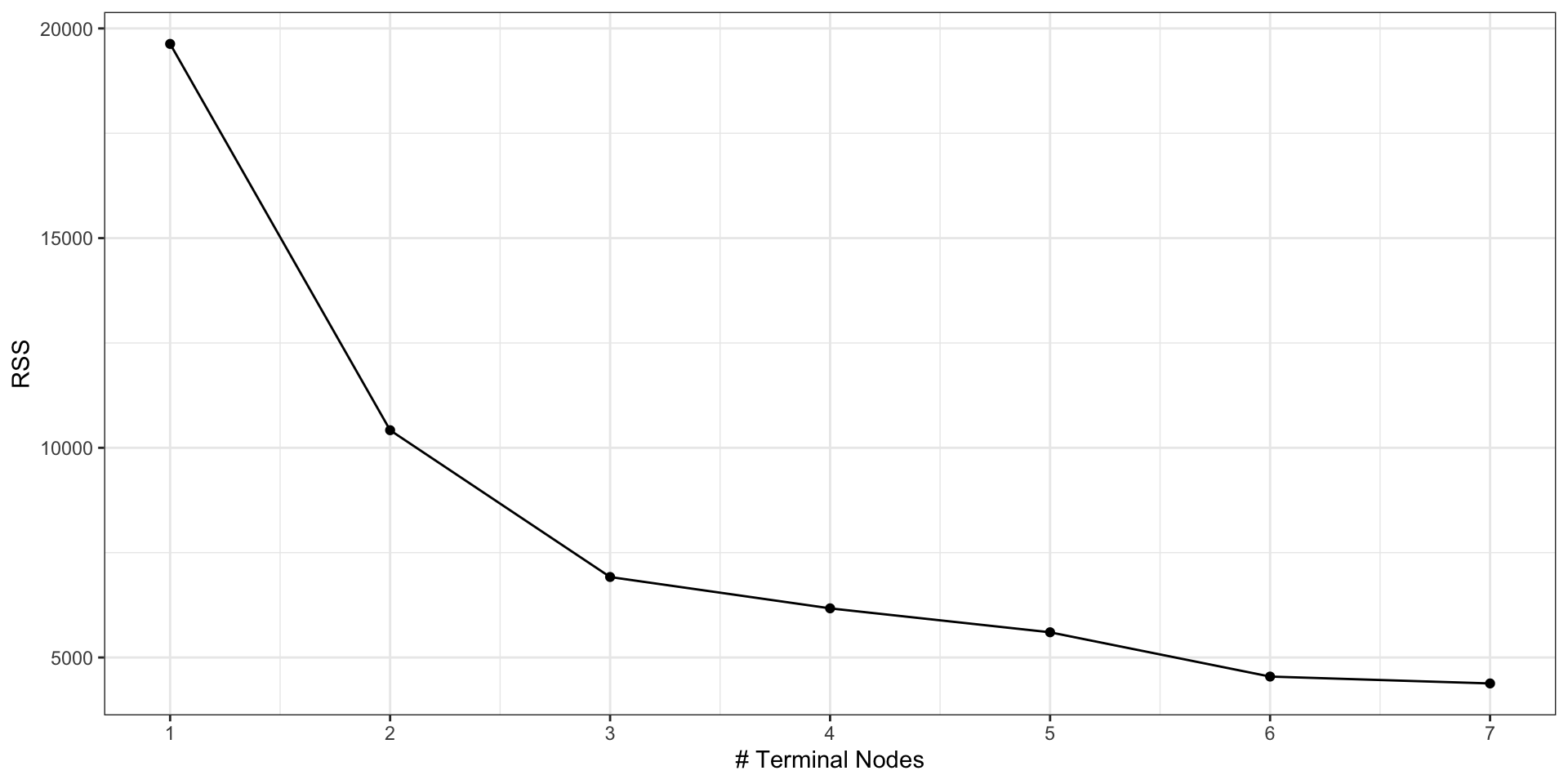
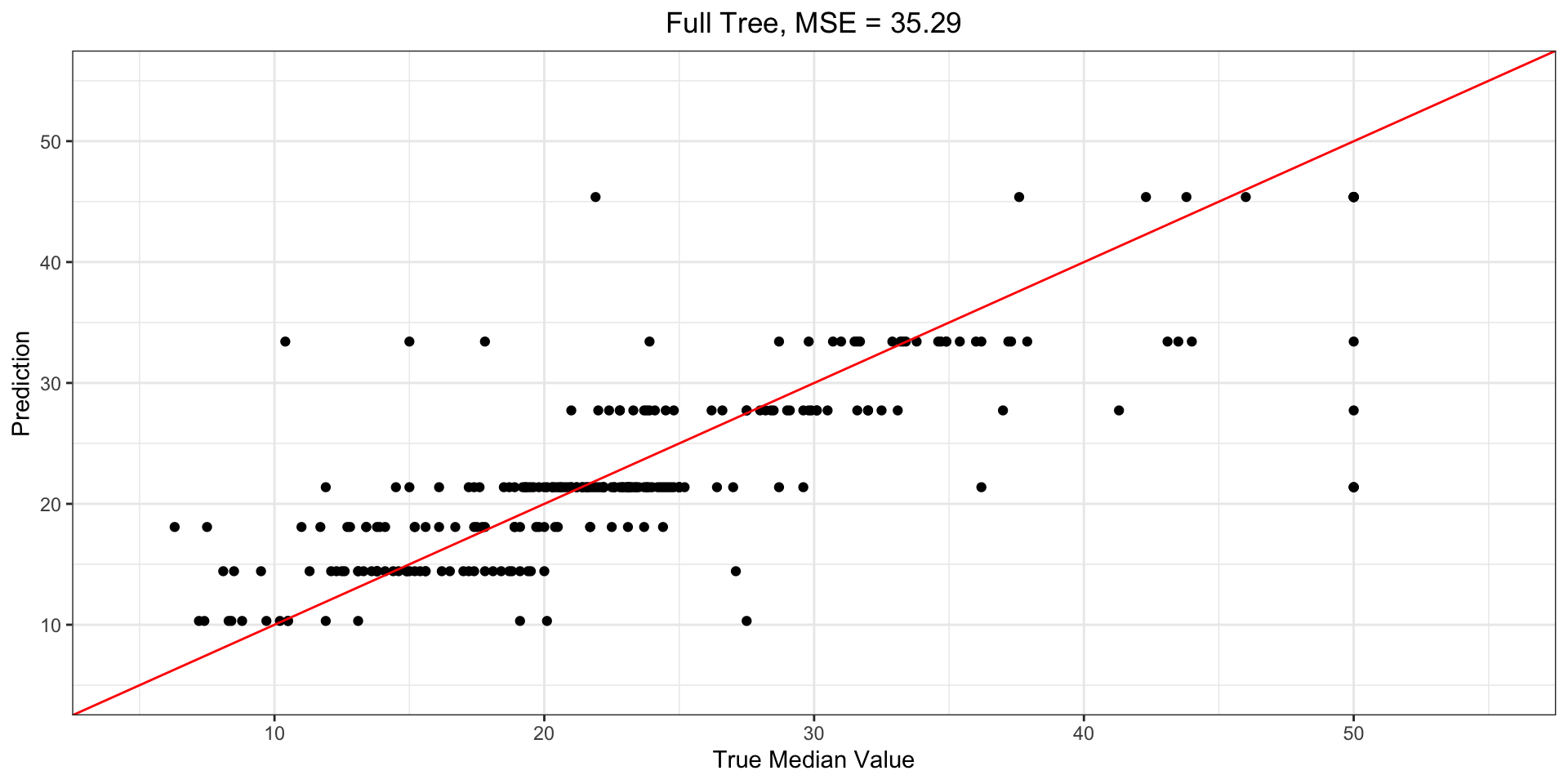
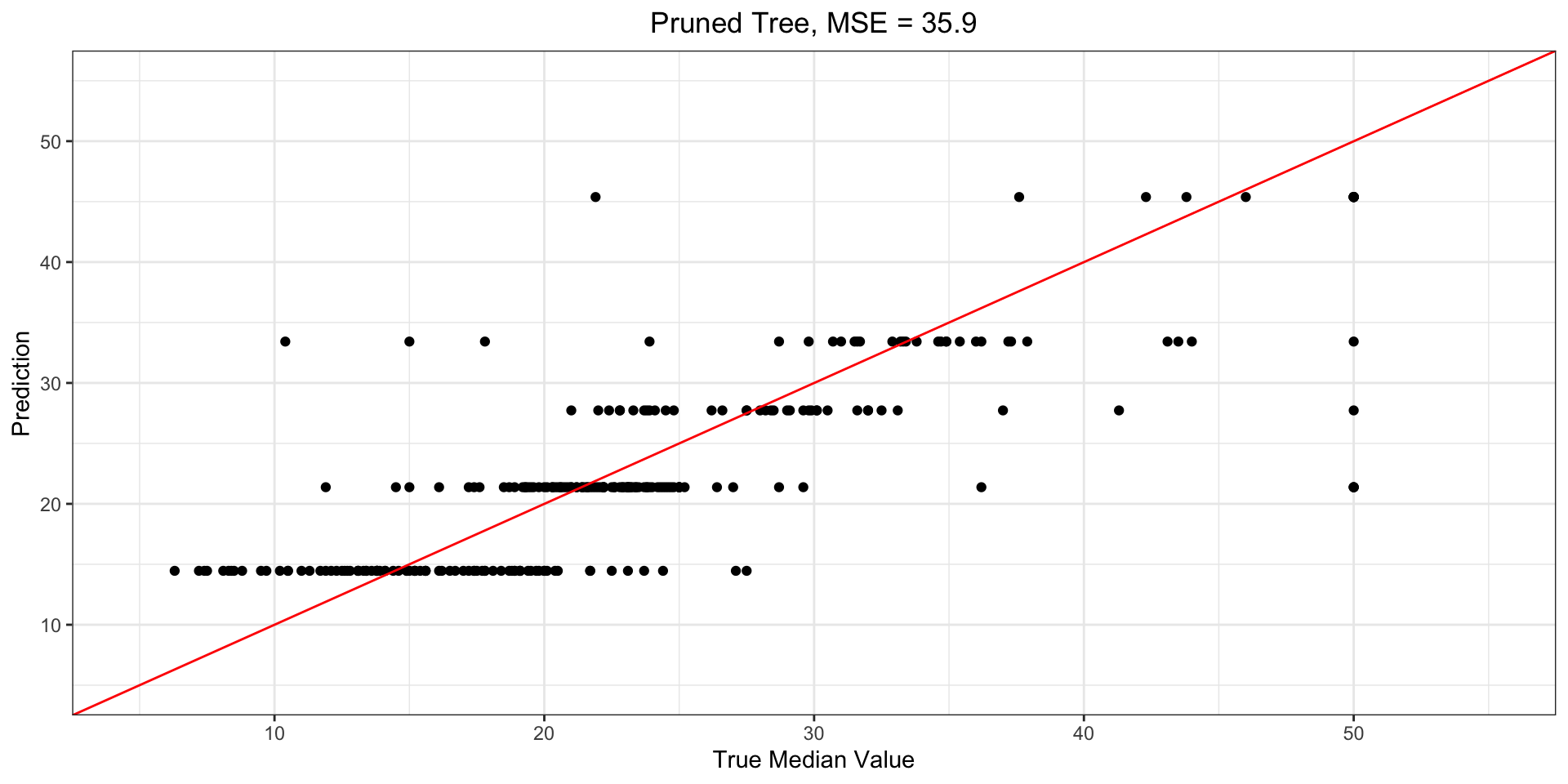
Even though the Cross-Validation shows that a 7-node tree minimizes the Cross-Validated RSS, we could still prune the tree:

prune_boston <- prune.tree(tree_boston, best = 5)
par(mar = rep(1,4))
plot(prune_boston)
text(prune_boston)

Predictions – Full Tree

yhat_boston_full <- predict(tree_boston, newdata = Boston[-boston_train , ])
boston_test <- Boston[-boston_train , "medv"]

Predictions – Pruned Tree

yhat_boston_prune <- predict(prune_boston, newdata = Boston[-boston_train , ])

Classification Trees

What do you think these are?

• A classification tree is very similar to a regression tree, except
  • it is used to predict a qualitative response rather than a quantitative one.
• Regression trees give a predicted response as the mean of the training observations that belong to a common region (terminal node);
• classification trees predict that each observation belongs to the most commonly occurring class of training observations in the region to which it belongs.

What Do We Use Them For?

In interpreting the results of a classification tree, we are often interested not only in the class prediction corresponding to a particular terminal node region, but also in the class proportions among the training observations that fall into that region.

For binary data, this is fairly simple, but it can scale up in complexity when dealing with factor/qualitative multi-level data.

How Do We Compute Them?

Everything is quite similar to regression trees, except we cannot use RSS in the recursive binary splitting. Instead, we use the classification error rate - the fraction of the training observations in a region that do not belong to the most common class.

\[ 1 - \underset{k}{\text{max}}\left( \hat{p}_{mk} \right) \]

It turns out this isn’t quite sensitive enough for tree-growing, so we use entropy, \[ D = - \sum_{k=1}^{K} \hat{p}_{mk} \log \hat{p}_{mk}. \] to determine the appropriate greedy choice for tree-growing.

A Note on Qualitative Predictors

We can split qualitative predictors in similar fashion to quantitative ones:

• Instead of splitting on a splitpoint \(s\), we instead group the levels of the factor into two branches, so that some of the levels go to one branch, and the rest to the other branch.
• This is still a partition.

An Example

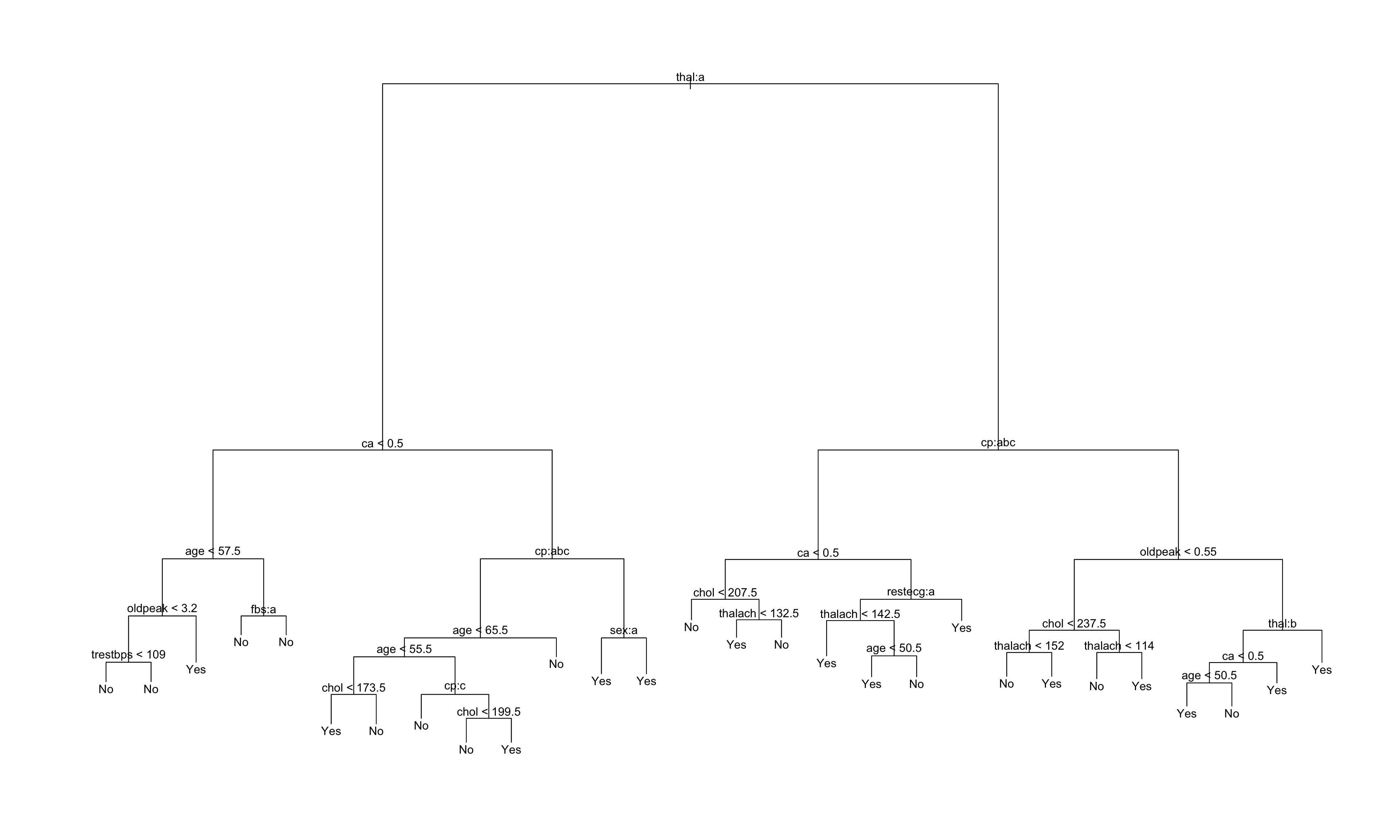
Heart disease data:

• binary outcome HD for 303 patients presenting with chest pain
  • Yes means heart disease based on an angiogram;
  • No means … no heart disease.
• Thal and ChestPain are qualitative predictors
  • On the next slide: the top node is Thal:a, which indicates the left branch is observations with the first level of Thal (‘Normal’), and the right is the remaining (‘Fixed or Reversible Defects’).

Heart Disease Tree

Node Purity

Some of the splits result in terminal nodes with the same predicted value.

• These splits are performed because they lead to increased node purity:
  • if one branch leads to a terminal node (leaf) which are all Yes (or No), while the other leads to a mixture which is still predominantly Yes (or No), you can have identical predictions.
• What differs is our level of certainty: one branch is highly certain, and one is somewhat uncertain.

Example: Carseat Sales

A simulated data set containing sales of child car seats at 400 different stores. We recode the continuous Sales variable into a binary variable.

data(Carseats)
Carseats <- Carseats |> 
  mutate(High = factor(ifelse(Sales <= 8, "No", "Yes")))
tree_carseats <- tree(High ~ . -Sales, data = Carseats)
summary(tree_carseats)

Classification tree:
tree(formula = High ~ . - Sales, data = Carseats)
Variables actually used in tree construction:
[1] "ShelveLoc"   "Price"       "Income"      "CompPrice"   "Population" 
[6] "Advertising" "Age"         "US"         
Number of terminal nodes:  27 
Residual mean deviance:  0.4575 = 170.7 / 373 
Misclassification error rate: 0.09 = 36 / 400 

Carseats: Interpreting

The residual mean deviance reported in the above is related to the entropy, with smaller levels indicating trees that provide a good fit to the training data.

There are 27 terminal nodes in this initial fit, which is perhaps a bit high.

Carseats: Plotting

par(mar = rep(1,4))
plot(tree_carseats)
text(tree_carseats)

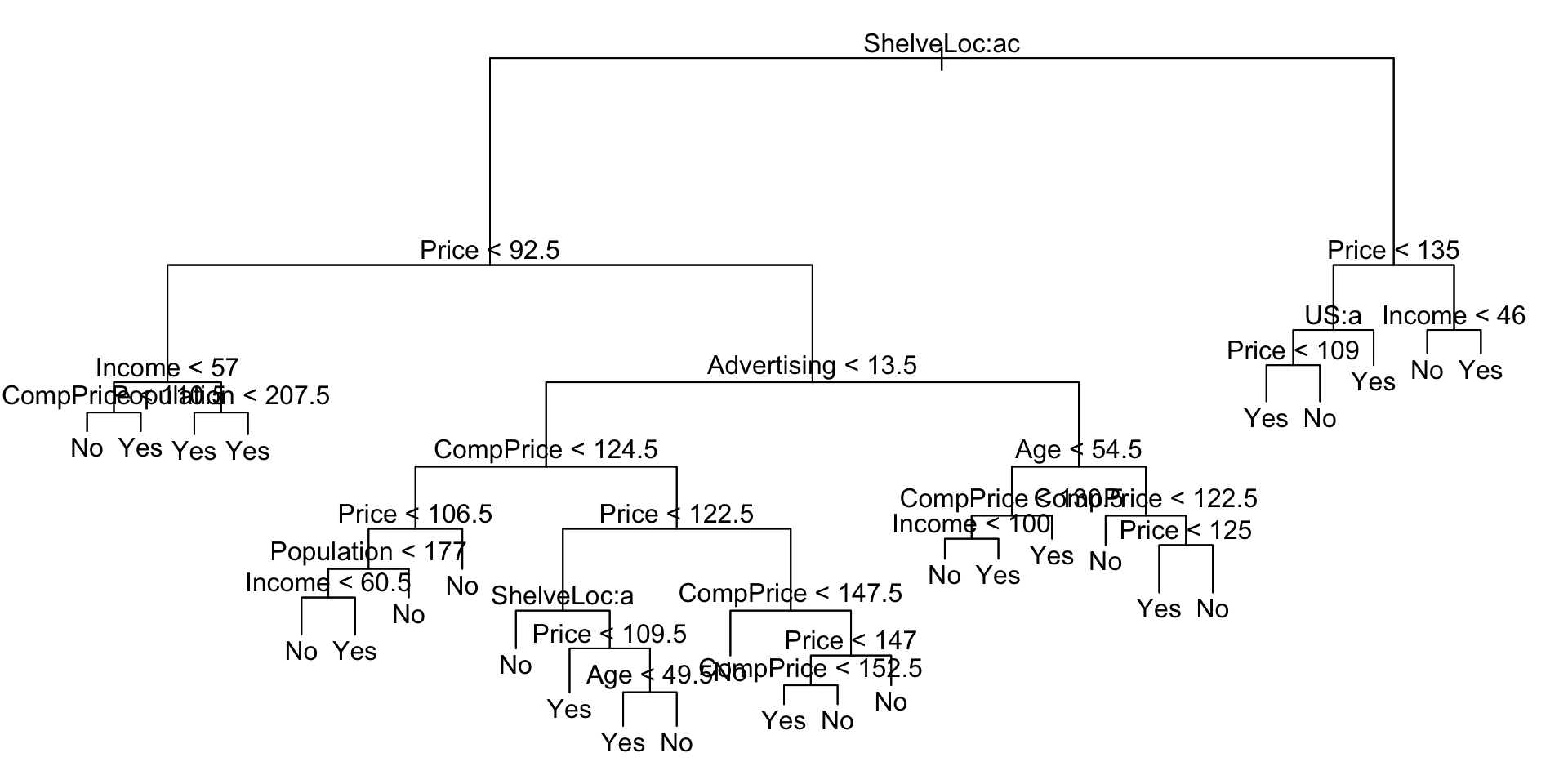
Carseats: Interpretations

• A note on the branch length:
  • longer branches indicate larger decreases in impurity, so they give a visual indication of how important a branch/node is in the overall predictor error reduction.
• The most important indicator of Sales seems to be shelving location, as we see from the first node.

Carseats: Estimating Test Error

We split the observations into a training set and a test set, build the tree using the training set, and evaluate its performance on the test data - around 77% correct.

set.seed(2)
carseat_train <- sample(1:nrow(Carseats), 200)
Carseats.test <- Carseats[-carseat_train, ]
High.test <- Carseats.test$High
tree.carseats <- tree(High ~ . -Sales, Carseats,
                      subset = carseat_train)
tree.pred <- predict(tree.carseats, Carseats.test,
                     type = "class")

Accuracy on Full (Unpruned) Tree

library(caret)
confusionMatrix(data = tree.pred, reference = High.test, positive = "Yes")

Confusion Matrix and Statistics

          Reference
Prediction  No Yes
       No  104  33
       Yes  13  50
                                          
               Accuracy : 0.77            
                 95% CI : (0.7054, 0.8264)
    No Information Rate : 0.585           
    P-Value [Acc > NIR] : 2.938e-08       
                                          
                  Kappa : 0.5091          
                                          
 Mcnemar's Test P-Value : 0.005088        
                                          
            Sensitivity : 0.6024          
            Specificity : 0.8889          
         Pos Pred Value : 0.7937          
         Neg Pred Value : 0.7591          
             Prevalence : 0.4150          
         Detection Rate : 0.2500          
   Detection Prevalence : 0.3150          
      Balanced Accuracy : 0.7456          
                                          
       'Positive' Class : Yes             
                                          

Carseats: Estimating Test Error

Does pruning the tree give a better result?

set.seed(7)
cv.carseats <- cv.tree(tree.carseats, FUN = prune.misclass)

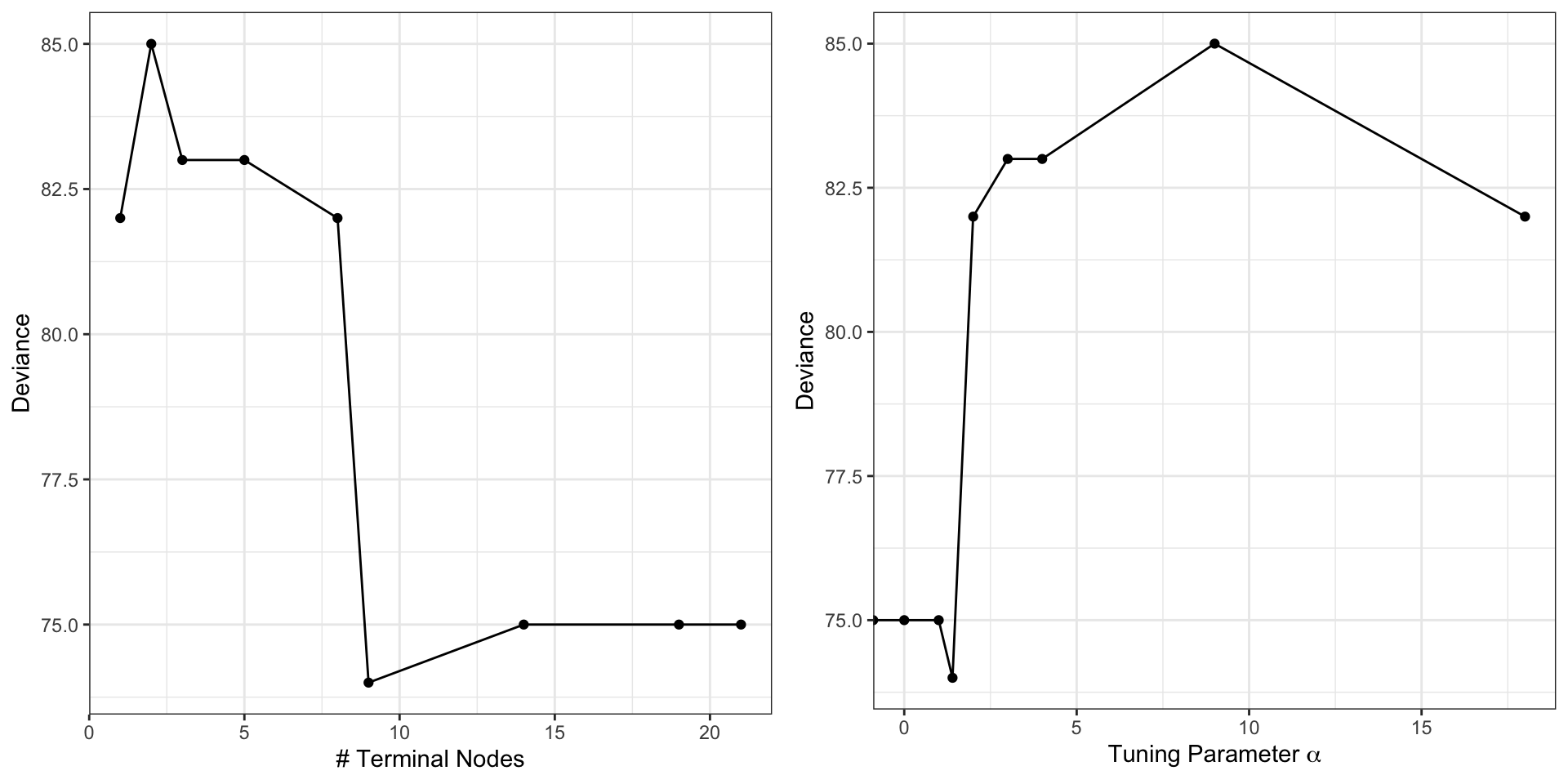
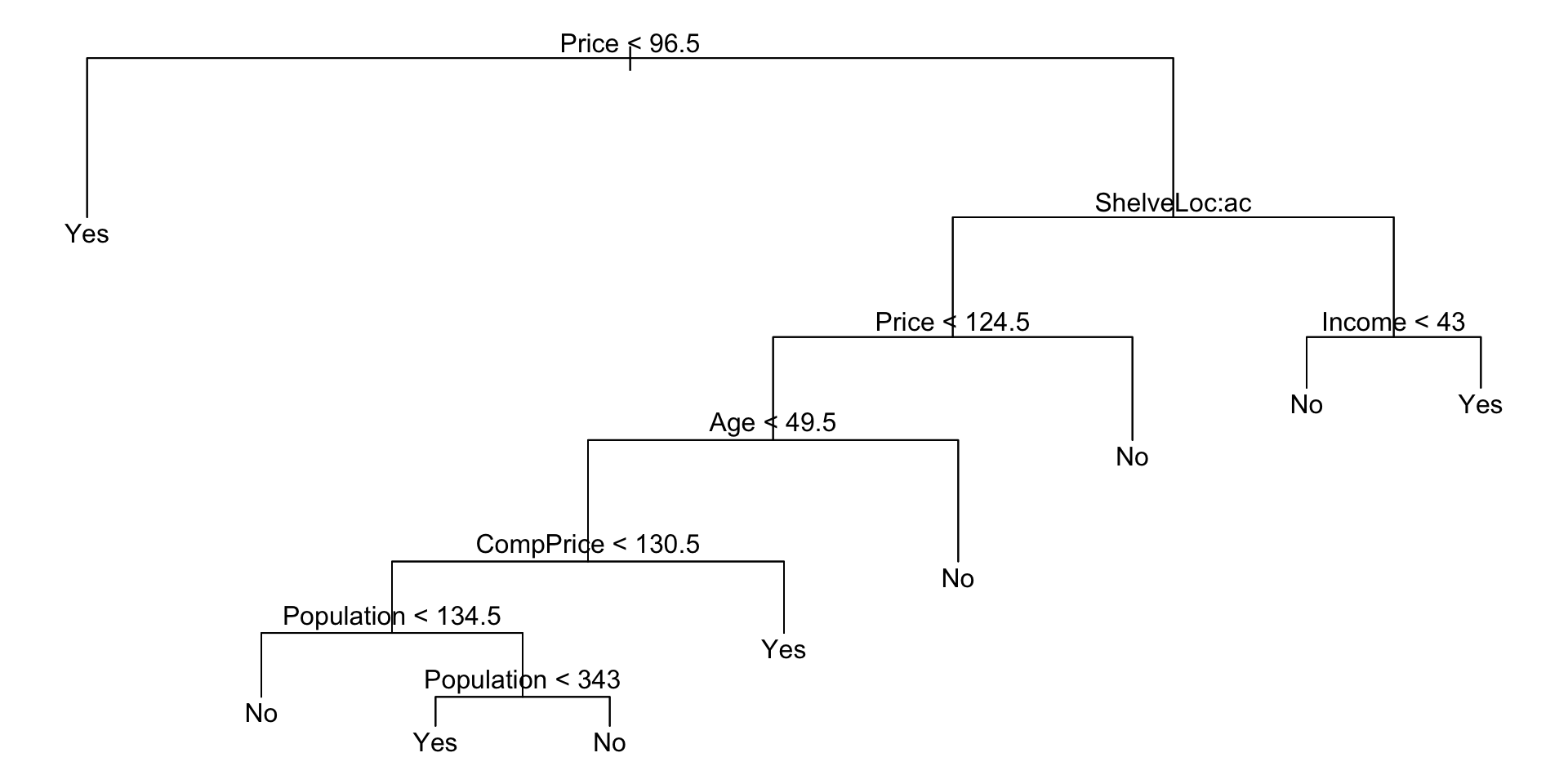
The Pruned Tree

prune.carseats <- prune.misclass(tree.carseats, best = 9)
par(mar = rep(1,4))
plot(prune.carseats)
text(prune.carseats)

Pruned Carseats: Estimating Test Error

The test accuracy is better and the tree is simpler!

tree.pred.prune <- predict(prune.carseats, Carseats.test, type = "class")
confusionMatrix(data = tree.pred.prune, reference = High.test, positive = "Yes")

Confusion Matrix and Statistics

          Reference
Prediction No Yes
       No  97  25
       Yes 20  58
                                          
               Accuracy : 0.775           
                 95% CI : (0.7108, 0.8309)
    No Information Rate : 0.585           
    P-Value [Acc > NIR] : 1.206e-08       
                                          
                  Kappa : 0.5325          
                                          
 Mcnemar's Test P-Value : 0.551           
                                          
            Sensitivity : 0.6988          
            Specificity : 0.8291          
         Pos Pred Value : 0.7436          
         Neg Pred Value : 0.7951          
             Prevalence : 0.4150          
         Detection Rate : 0.2900          
   Detection Prevalence : 0.3900          
      Balanced Accuracy : 0.7639          
                                          
       'Positive' Class : Yes             
                                          

Ensemble Improvements

Ensemble Methods

• An ensemble method is an approach that combines many simple “building block” models in order to obtain a single and potentially very powerful model.
  • These simple building block models are sometimes known as weak learners, since they may lead to mediocre predictions on their own.
• There are four different ensemble methods which use as their inputs simple regression or classification trees:
  • bagging
  • boosting
  • random forests
  • Bayesian additive regression trees (BART)

Bagging

Bagging

• Remember the (very!) brief introduction to the bootstrap we did two weeks ago? Bagging uses the bootstrap to improve decision trees.

• The decision trees we discussed earlier suffer from high variance: if we split the data into two parts, completely at random, we could get wildly different predictions from the two halves.

• Bootstrap aggregation (b-agg’ing, or bagging), is a procedure for reducing the variance of a statistical learning method, particularly useful for trees.

Bagging: How Does It Work?

• In statistics, if we have a set of \(n\) independent observations, \(X_1, \cdots, X_n\), with common variance \(\sigma^2\), then the variance of the mean \(\bar{X}\) is \(\sigma^2/n\).
• Averaging a set of observations reduces the variance.
• So what if we took many different training sets from the population, built separate prediction models using each, and averaged the predictions?
• This is not practical because we do not have access to multiple training sets. But we could … bootstrap!

Bagging: How Does It Work?

1. Generate \(B\) different bootstrapped training data sets
2. Train the method on each bootstrapped training set
3. Average all of the predictions

This process is called bagging.

So far, this process is for quantitative outcomes - regression trees.

Bagging: Qualitative Response

• For a qualitative \(Y\), we record the class predicted by each of the \(B\) trees
• We then take majority vote across the bootstrap replicated trees
• The overall prediction is the most commonly occurring class among the \(B\) predictions.

Bagging: Test Errors

• We need some way of estimating the test error of a bagged model.
  • Remember: trees are fit to bootstrapped subsets of the observations.
• It turns out that this bootstrap procedure results in each tree being fit on around 2/3 of the observations
  • the remaining 1/3 can be used to test, and referred to as the Out-of-Bag (OOB) observations.
• So if all trees for which a given observation is OOB have their predictions averaged or majority voted, we get a single OOB prediction for each observation.
  • This can be repeated for every observation.

Bagging: Test Errors

• The resulting OOB MSE or OOB classification error can be computed on these \(n\) OOB predictions, giving a result which can be interpreted.
• Advantage of this approach: as \(B\) grows, the OOB approach converges to the same result as doing LOOCV, which is highly computationally demanding for trees.
  • As always … let the computer do the work!

Random Forests

Random Forests

• Random forests provide an improvement over bagged trees by way of a small tweak that decorrelates the trees.
• As in bagging, we build a number of decision trees on bootstrapped training samples.
• But when building these decision trees, each time a split in a tree is considered, a random sample of \(m\) predictors is chosen as split candidates from the full set of \(p\) predictors.
• The split is allowed to use only one of those \(m\) predictors.
• A fresh sample of \(m\) predictors is taken at each split
  • typically we choose \(m \approx \sqrt{p}\).

Random Forests: What?

In other words, in building a random forest, at each split in the tree, the algorithm is not even allowed to consider a majority of the available predictors.

This may sound crazy, but it has a clever rationale:

• Suppose that there is one very strong predictor in the data set, along with a number of other moderately strong predictors.
• Then in the collection of bagged trees, most or all of the trees will use this strong predictor in the top split.
• Consequently, all of the bagged trees will look quite similar to each other.

Random forests overcome this by forcing each split to consider only a subset of the predictors - making the average less variable, and hence more reliable.

Random Forests: Compared to Previous

• The main difference between bagging and random forests is the choice of the subset size \(m\).
• If \(m=p\), then this process is just bagging.
• Choosing a smaller \(m\), say \(m = \sqrt{p}\), can result in a reduction in both test error and OOB error over bagging.
• As with bagging, random forests will not overfit if we increase \(B\), so in practice we use a value of \(B\) sufficiently large for the error rate to have “settled down”

Boosting

Boosting

• Like bagging, boosting is a general approach that can be applied to many statistical learning methods for regression or classification.
  • Here we restrict our discussion of boosting to the context of decision trees.
• In bagging, we create multiple copies of the original training data using the bootstrap, fit separate decision trees, then combine the trees to create a single predictive model.
• Boosting is similar, except the trees are grown sequentially:
  • each tree is grown using information from the previous
  • no bootstrap, just modifications to the observed data at each stage

Boosting: The Idea

• Unlike fitting a single large decision tree to the data
  • this amounts to fitting the data hard and potentially overfitting
  • the boosting approach instead learns slowly
    • given the current model, we fit a decision tree to the residuals from the model.
• We fit a tree using the current residuals, rather than the outcome \(Y\), as the response.
• We then add this new decision tree into the fitted function in order to update the residuals.
• Each of these trees can be rather small, with just a few terminal nodes, determined by the parameter \(d\) in the algorithm.

Boosting: The Idea

• By fitting small trees to the residuals, we slowly improve the model in areas where it does not perform well.
• The shrinkage parameter \(\lambda\) slows the process down even further, allowing more and different shaped trees to attack the residuals. In general, statistical learning approaches that learn slowly tend to perform well.

Note that in boosting, unlike in bagging, the construction of each tree depends strongly on the trees that have already been grown.

Boosting: Parameters

There are three tuning parameters:

• the number of trees: \(B\)
  • use CV to choose
• shrinkage parameter, \(\lambda\) - rate at which boosting ‘learns’
  • typically small, between 0.01 and 0.001
  • values of \(\lambda\) that are too small will require a large \(B\)
• number of splits: \(d\)
  • controls complexity
  • more generally interaction depth
  • often \(d=1\) works well
    • the case of \(d=1\) is called a stump; just a single split

BART

Bayesian Additive Regression Trees (BART)

• Our final improvement method is Bayesian Additive Regression Trees (BART).
• In BART, each tree in the sequence is constructed in a random manner, like bagging and random forests, but each tree also tries to capture signal that hasn’t yet been accounted for, like boosting.

BART: How Does It Work?

1. To start, initialize \(K\) trees with a single root node
2. Update each of the \(K\) trees, one at a time, and for each iteration:
   • subtract from each response value the predictions from all but the \(k^{\text{th}}\) tree, obtaining a partial residual
3. Then, instead of fitting a fresh tree to this residual, as boosting might do, BART randomly chooses a perturbation to the tree, from a set of possible such perturbations, giving weight to the ones that improve the fit.
   • The perturbations are adding or pruning branches, or changing the prediction in each terminal node.

BART

Output?

The output of BART is then a set of prediction models for \(1, 2, \cdots, B\). Usually the first few are quite bad, and we throw them out - this is referred to as the burn-in period.

Key Advantage

The key advantage to BART over boosting is that because BART tries to improve the results at each step by slightly modifying the previous tree, it guards against overfitting because it limits how “hard” we can fit the data at each iteration. Smaller steps means slower, and slower is typically better.

BART: Parameters

When we fit a BART model, we have to choose the number of trees, \(K\), the number of iterations, \(B\), and the number of burn-in iterations, \(L\). Usually \(B\) and \(K\) are large, and \(L\) is moderate.

BART is nice because it has very good default performance, and requires minimal tuning usually to give decent predictions.

Examples of Ensemble Methods

Back to Boston, Bagging

We set mtry = 12 because there are 12 predictors in the dataset.

library(randomForest)
set.seed(1)
bag.boston <- randomForest(medv ~ ., data = Boston,
                           subset = boston_train, 
                           mtry = 12, importance = TRUE)
bag.boston

Call:
 randomForest(formula = medv ~ ., data = Boston, mtry = 12, importance = TRUE,      subset = boston_train) 
               Type of random forest: regression
                     Number of trees: 500
No. of variables tried at each split: 12

          Mean of squared residuals: 11.40162
                    % Var explained: 85.17

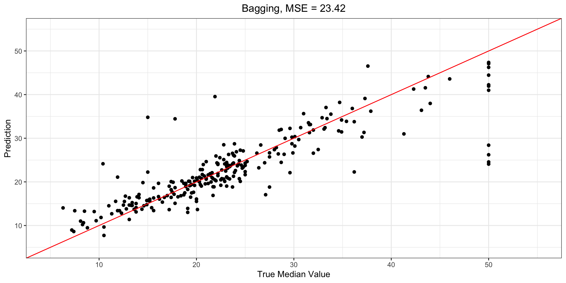
Boston, Recall

yhat_boston_bag <- predict(bag.boston, newdata = Boston[-boston_train, ])

Boston, Compare

So we have

errors <- bind_rows(
  data.frame(method = "Pruned Tree", y = boston_test, yhat = yhat_boston_prune),
  data.frame(method = "Bagging",     y = boston_test, yhat = yhat_boston_bag)
) 

errors |> group_by(method) |> summarize(MSE = mean((y -yhat)^2)) |> arrange(MSE, desc = FALSE)

# A tibble: 2 × 2
  method        MSE
  <chr>       <dbl>
1 Bagging      23.4
2 Pruned Tree  35.9

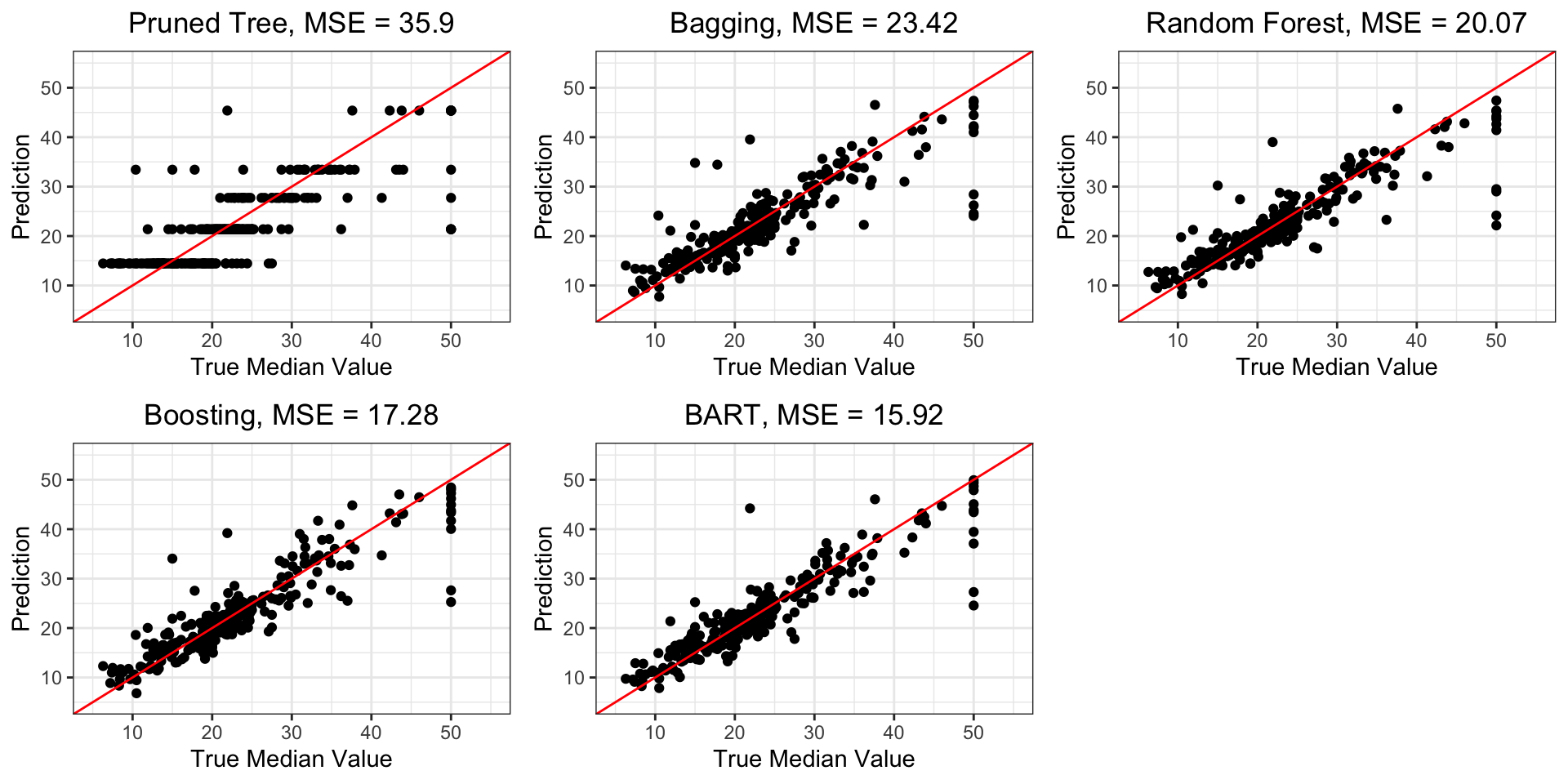
a reduction in MSE by about 1/3: the previous optimally-pruned single tree had a MSE of around 36, and we now have around 23.

Boston, Random Forest

If we don’t set mtry to 12, we get an actual random forest model:

set.seed(1)
rf.boston <- randomForest(medv ~ ., data = Boston,
                          subset = boston_train, mtry = 6, importance = TRUE)
yhat_boston_rf <- predict(rf.boston, newdata = Boston[-boston_train, ])

# A tibble: 3 × 2
  method          MSE
  <chr>         <dbl>
1 Random Forest  20.1
2 Bagging        23.4
3 Pruned Tree    35.9

So choosing from a random selection of 6 variables at each split, we get a random forest which slightly improves on the previous test MSE of the bagging model above.

Boston, Random Forest

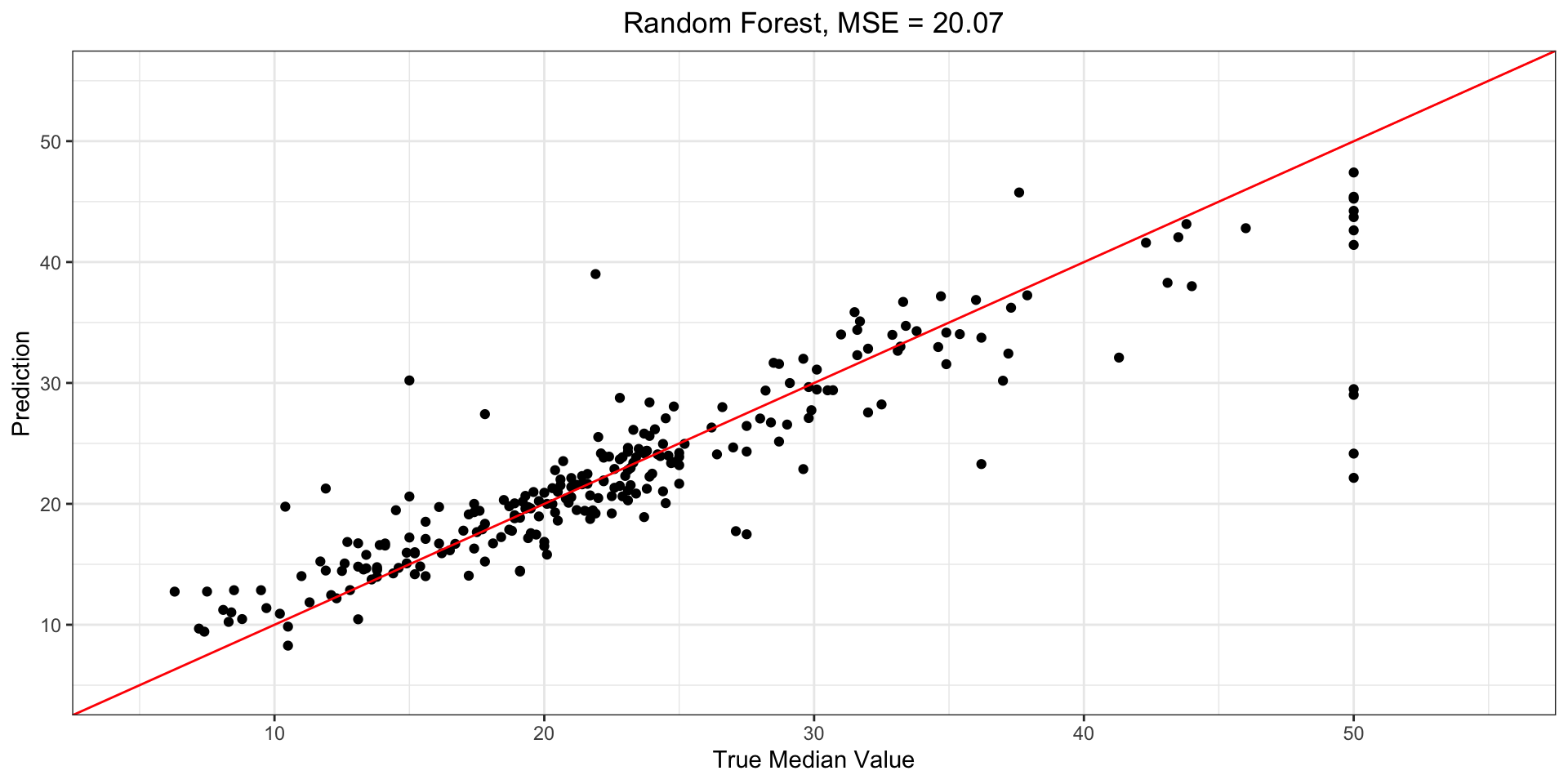
Boston, Random Forest

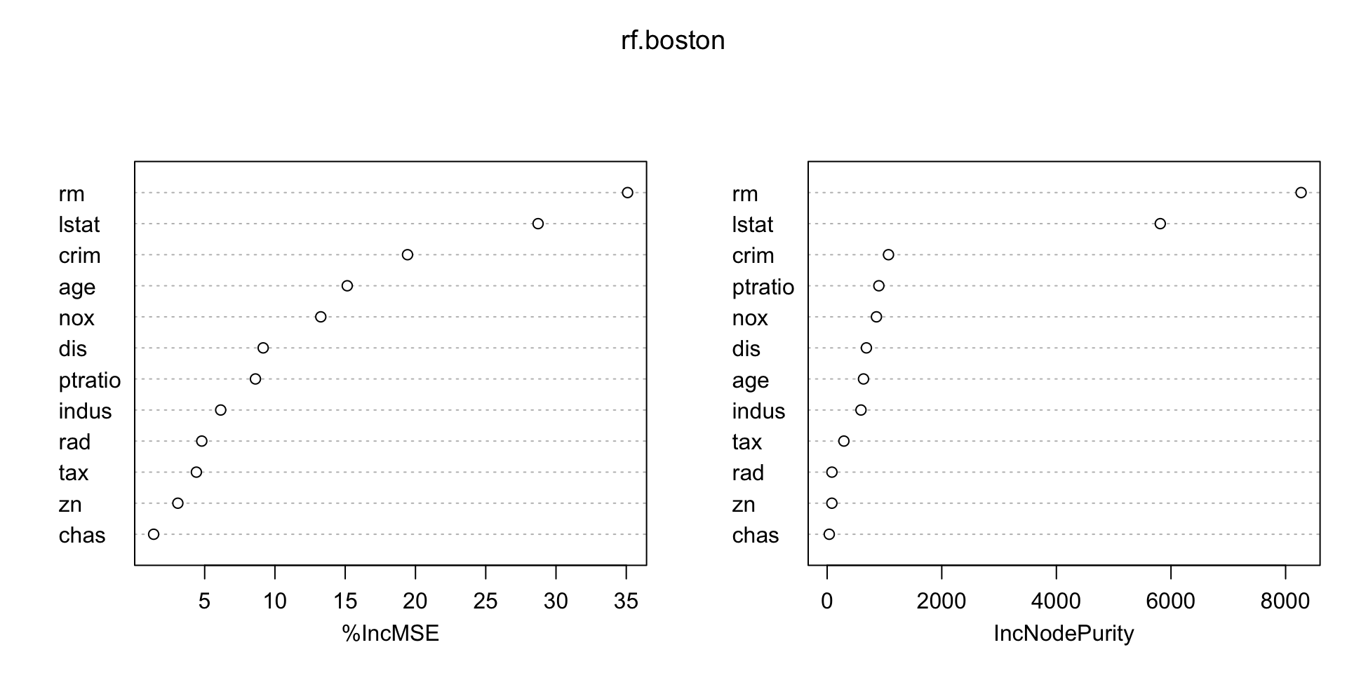
We can look at the importance of each variable:

importance(rf.boston)

          %IncMSE IncNodePurity
crim    19.435587    1070.42307
zn       3.091630      82.19257
indus    6.140529     590.09536
chas     1.370310      36.70356
nox     13.263466     859.97091
rm      35.094741    8270.33906
age     15.144821     634.31220
dis      9.163776     684.87953
rad      4.793720      83.18719
tax      4.410714     292.20949
ptratio  8.612780     902.20190
lstat   28.725343    5813.04833

Boston, Random Forest

We can also plot, showing lstat (wealth) and rm (house size) are by far the most important.

varImpPlot(rf.boston)

Boston, Boosting

Another new package, gbm.

library("gbm")
set.seed(1)
boost.boston <- gbm(medv ~ ., data = Boston[boston_train, ],
                    distribution = "gaussian", n.trees = 5000,
                    interaction.depth = 4, cv.folds = 10)

Boston, Boosting

summary(boost.boston, 
        plotit = FALSE)

            var      rel.inf
rm           rm 44.936598303
lstat     lstat 29.812159051
crim       crim  6.103055959
dis         dis  4.762815179
nox         nox  4.335382715
age         age  3.761324798
tax         tax  2.288495519
ptratio ptratio  2.279678246
indus     indus  0.953981946
rad         rad  0.632964710
zn           zn  0.131312988
chas       chas  0.002230587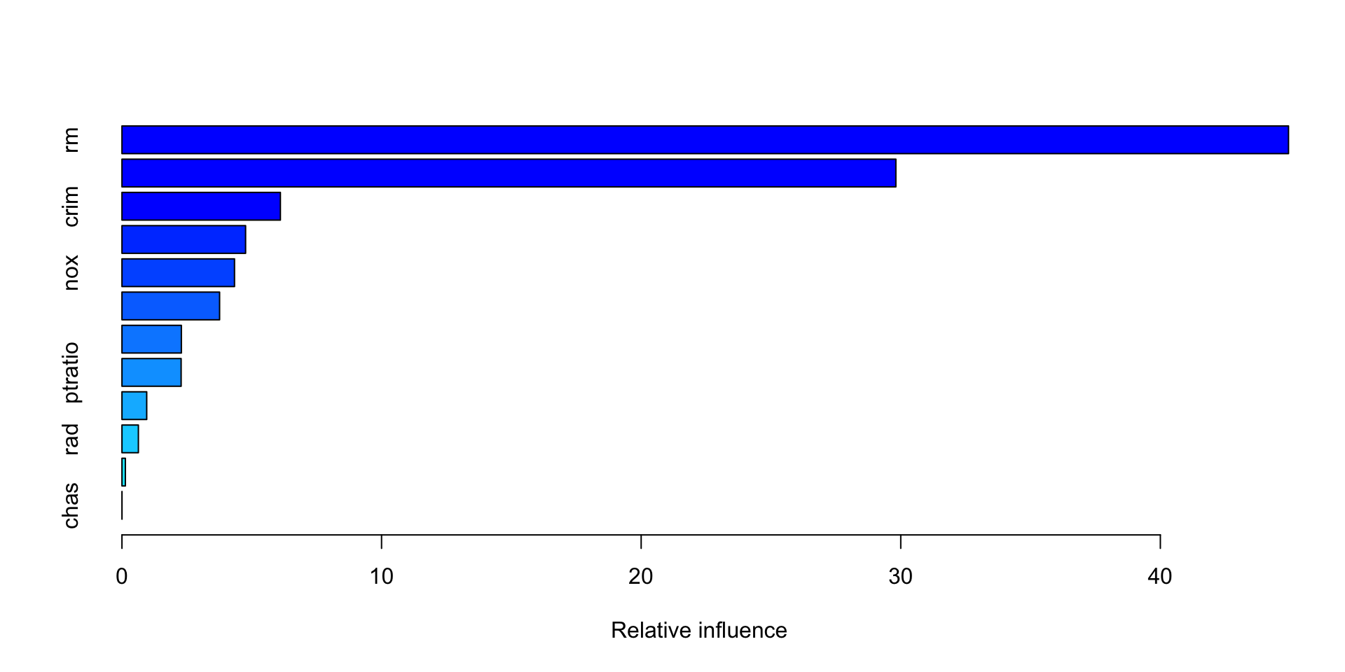

invisible(summary(boost.boston))

Boston, Boosting

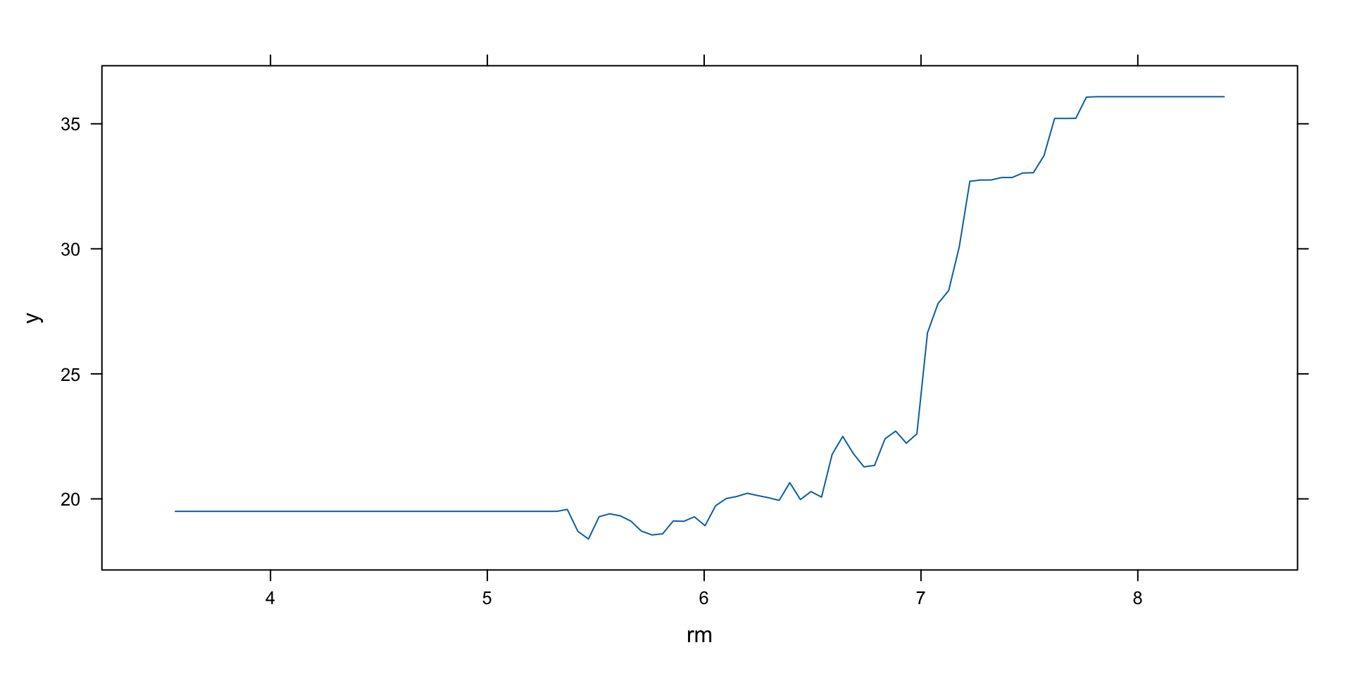
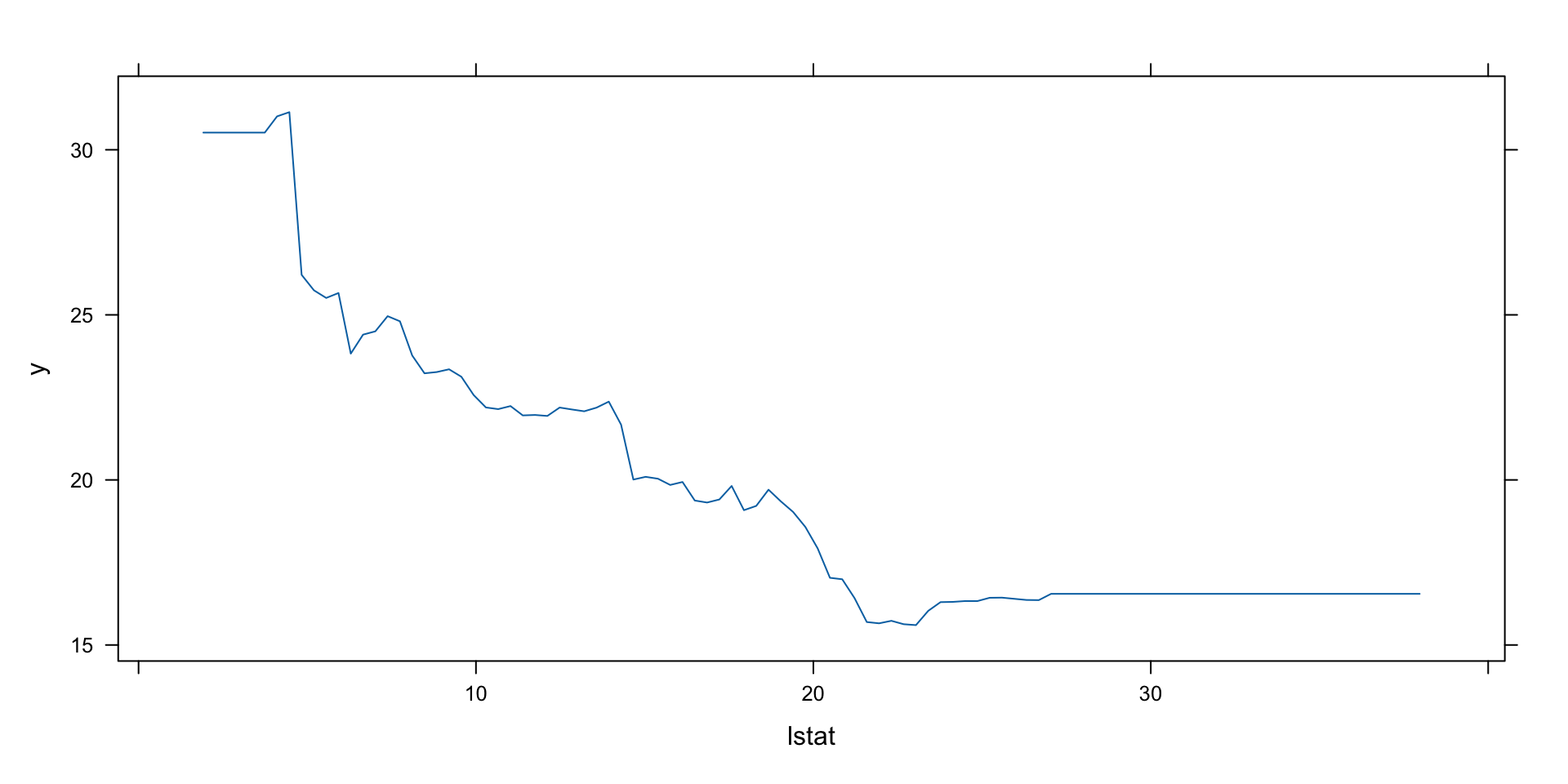
Again, lstat and rm are the most important variables by far. We can plot the partial dependence plot, which shows that medv (median house prices) are increasing with rm.

Boston, Boosting

Median house prices decrease with lstat.

Boston, Boosting, Predict

Using cross-validation, the best iteration was 361 trees.

print(boost.boston)

gbm(formula = medv ~ ., distribution = "gaussian", data = Boston[boston_train, 
    ], n.trees = 5000, interaction.depth = 4, cv.folds = 10)
A gradient boosted model with gaussian loss function.
5000 iterations were performed.
The best cross-validation iteration was 361.
There were 12 predictors of which 11 had non-zero influence.

yhat_boston_boost <- predict(boost.boston,
                      newdata = Boston [-boston_train, ], n.trees = 361)

# A tibble: 4 × 2
  method          MSE
  <chr>         <dbl>
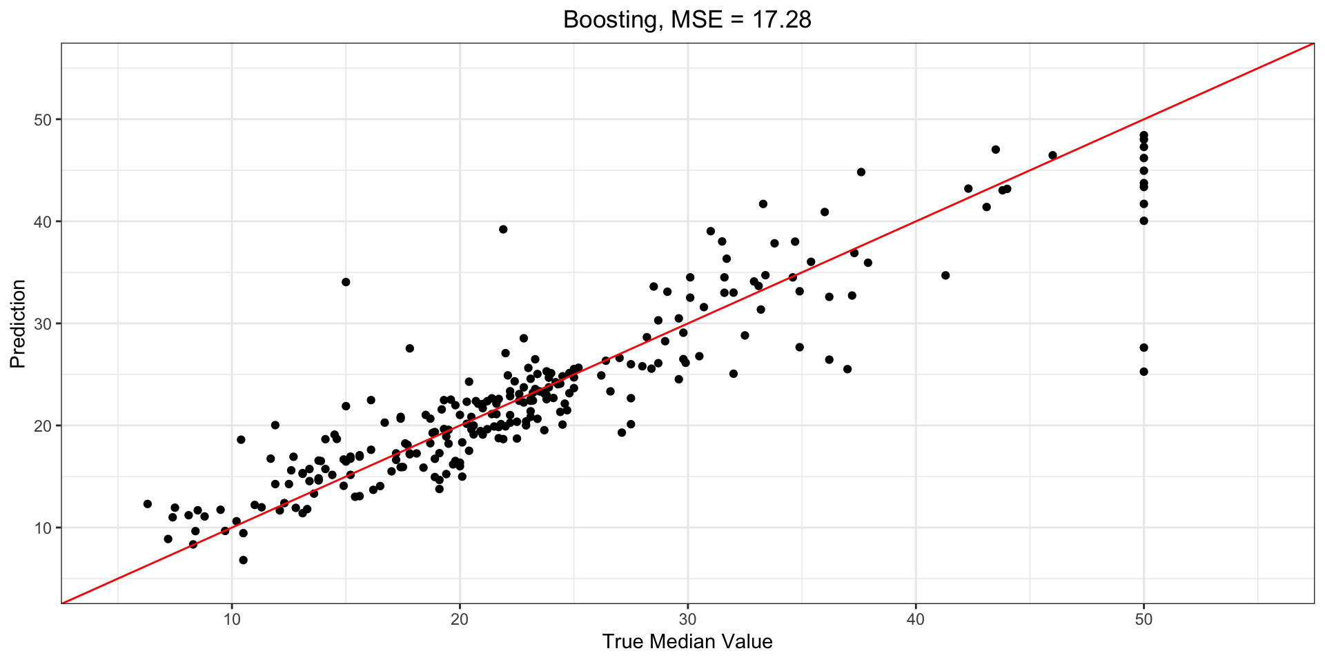
1 Boosting       17.3
2 Random Forest  20.1
3 Bagging        23.4
4 Pruned Tree    35.9

Significant improvement again, over both bagging and random forest.

Boston, Boosting

Boston, BART

library(BART)
x <- Boston[, 1:12]
y <- Boston[ , "medv"]
xtrain <- x[boston_train, ]
ytrain <- y[boston_train]
xtest <- x[-boston_train, ]
ytest <- y[-boston_train]
set.seed(1)
bart_fit <- gbart(xtrain, ytrain, x.test = xtest)

*****Calling gbart: type=1
*****Data:
data:n,p,np: 253, 12, 253
y1,yn: 0.213439, -5.486561
x1,x[n*p]: 0.109590, 20.080000
xp1,xp[np*p]: 0.027310, 7.880000
*****Number of Trees: 200
*****Number of Cut Points: 100 ... 100
*****burn,nd,thin: 100,1000,1
*****Prior:beta,alpha,tau,nu,lambda,offset: 2,0.95,0.795495,3,3.71636,21.7866
*****sigma: 4.367914
*****w (weights): 1.000000 ... 1.000000
*****Dirichlet:sparse,theta,omega,a,b,rho,augment: 0,0,1,0.5,1,12,0
*****printevery: 100

MCMC
done 0 (out of 1100)
done 100 (out of 1100)
done 200 (out of 1100)
done 300 (out of 1100)
done 400 (out of 1100)
done 500 (out of 1100)
done 600 (out of 1100)
done 700 (out of 1100)
done 800 (out of 1100)
done 900 (out of 1100)
done 1000 (out of 1100)
time: 1s
trcnt,tecnt: 1000,1000

Boston, BART

We can check how many times each variable appeared in the collection of trees.

ord <- order (bart_fit$varcount.mean, decreasing = TRUE)
bart_fit$varcount.mean[ord]

    nox   lstat     rad      rm     tax ptratio    chas     age   indus      zn 
 22.973  21.653  21.638  20.725  20.021  19.615  19.283  19.278  19.073  15.576 
    dis    crim 
 13.800  11.607 

Recall that BART is randomizing the selection, to try to ensure we don’t overfit. Notice how rm and lstat are not the highest, despite being the most important predictors by far in the earlier model? This is BART acting to keep us from overfitting by forcing all models to start with these two.

Boston, BART

Boston, BART

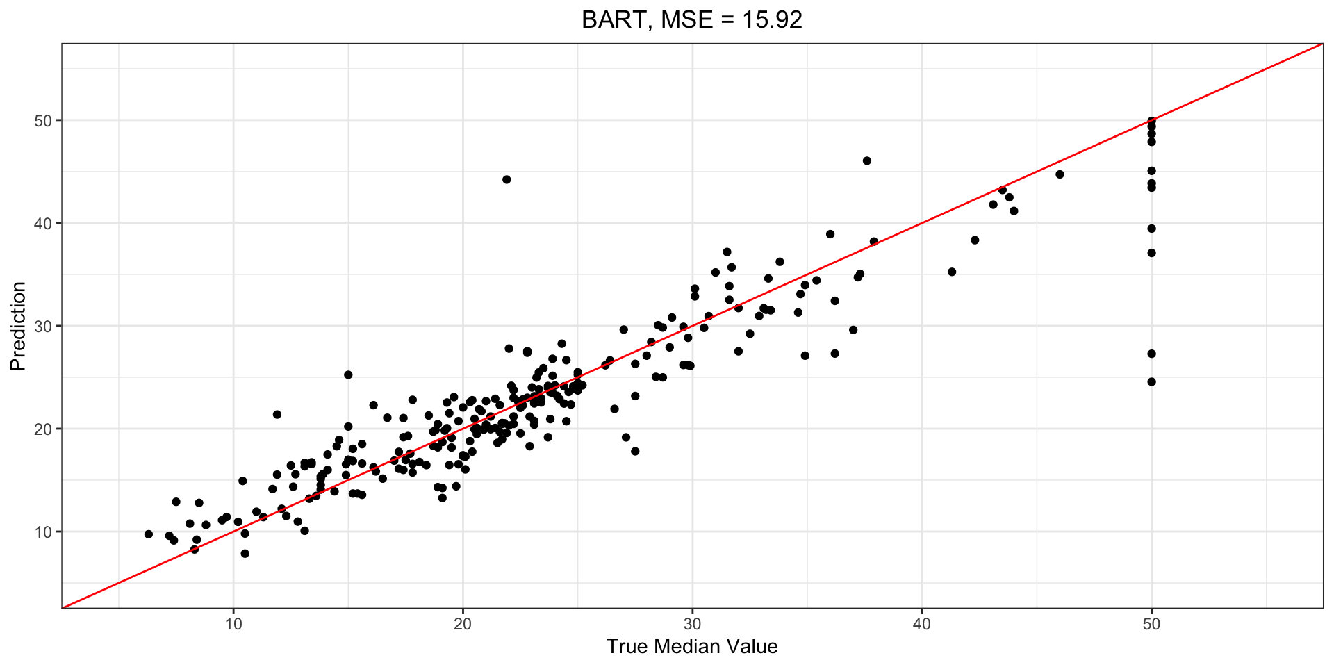
We can compute the error, again:

yhat_boston_bart <- bart_fit$yhat.test.mean

# A tibble: 5 × 2
  method          MSE
  <chr>         <dbl>
1 BART           15.9
2 Boosting       17.3
3 Random Forest  20.1
4 Bagging        23.4
5 Pruned Tree    35.9

So on this data set, the BART result is the best for MSE on the test data.

Actual vs Fitted Plots

Summary

Trees are an attractive choice of weak learner for an ensemble method for a number of reasons, including their flexibility and ability to handle predictors of mixed types (i.e., qualitative as well as quantitative). We have now seen four approaches for fitting an ensemble of trees: bagging, random forests, boosting, and BART.

• in bagging, the trees are grown independently on random samples, so the trees tend to be pretty similar. Thus, bagging can get ‘caught’ on local minimums and maximums, and fail to fully explore the model space.

Summary

• in boosting, we only use the original data, no random samples. But the trees are grown “slowly”, learning on the signal left over from previous trees, and shrunk before used.
• in random forests, trees are grown independently on random samples of the observations, but the splits are done using a random subset of the features, resulting a more thorough exploration of the model space relative to bagging.
• finally, in BART, we again make use only of the original data, and grow trees successively, but each tree is perturbed in order to avoid local minima, and achieve a more thorough exploration of the model space.

Summary: New Packages

New packages used today are:

• tree: general tree utility, non-ensemble methods
• randomForest: random forests and bagging
• gbm: Boosting
• BART: Bayesian Additive Regression Trees

Next Topics

After Reading Week, we will do the final two topics from ISLR2: Support Vector Machines and Deep Learning. The latter will be a very high-level overview of a topic that could be an entire course (and often is multiple courses, see, e.g., some of the COIS offerings at Trent).

Readings

The material of this week is Chapters 8.1-8.2 of ISLR2, discussing tree-based methods.

Readings for the two weeks following reading week are Chapters 9.1-9.5 for week 8, and 10.1-10.7 for the following, week 9.