Rows: 10,000
Columns: 4
$ default <fct> No, No, No, No, No, No, No, No, No, No, No, No, No, No, No, No…
$ student <fct> No, Yes, No, No, No, Yes, No, Yes, No, No, Yes, Yes, No, No, N…
$ balance <dbl> 729.5265, 817.1804, 1073.5492, 529.2506, 785.6559, 919.5885, 8…
$ income <dbl> 44361.625, 12106.135, 31767.139, 35704.494, 38463.496, 7491.55…Lecture 03 – Classification
AMOD-5440
Kat Clark
Trent University
2026-09-25
Extending the Linear Model to Logistic
Linear Models
- Regression is a short-hand for the general class of linear models where the response is related to a linear combination of predictors via equality: \[ Y = f(X) = \beta_0 + \sum_{j=1}^{p} \beta_j x_j + \varepsilon \]
- This model allows \(p\) predictors \(X\) to be combined via addition, and scalar multiplication, to model an observed \(Y\), with additive noise \(\varepsilon\). In simpest form, this is simple linear regression, where \(y = \beta_0 + \beta_1 x + \varepsilon.\)
New Idea
- The linear regression model from earlier assumes that the response variable \(Y\) is quantitative.
- But in many situations, the response variable is instead qualitative.
- For example, eye color is qualitative. Often qualitative variables are referred to as categorical.
- Predicting such responses is known as classification.
Why Classification?
- Predicting a qualitative response for an observation can be referred to as classifying that observation, since it involves assigning the observation to a category, or class.
- On the other hand, often the methods used for classification first predict the probability that the observation belongs to each of the categories of a qualitative variable, as the basis for making the classification.
- In this sense they also behave like regression methods.
Some Examples
- A person arrives at the emergency room with a set of symptoms that could possibly be attributed to one of three medical conditions. Which of the three conditions does the individual have?
- An online banking service must be able to determine whether or not a transaction being performed on the site is fraudulent, on the basis of the user’s IP address, past transaction history, and so forth.
- A university admissions office wants to predict whether an applicant will accept or decline an offer of admission based on application and demographic information.
- A streaming service wants to classify a movie as belonging to one of several genres (e.g., comedy, drama, action, documentary) using information about its content.
Why Not Linear Regression?
Linear regression doesn’t work well for classification problems. But why not?
- Regression methods cannot accommodate a qualitative response with more than two classes
- Regression methods will not provide meaningful estimates of \(\Pr\left(Y | X \right)\), even with just two classes.
- Thus, it is preferable to use a classification method that is truly suited for qualitative response values.
Why Doesn’t Linear Regression Work?
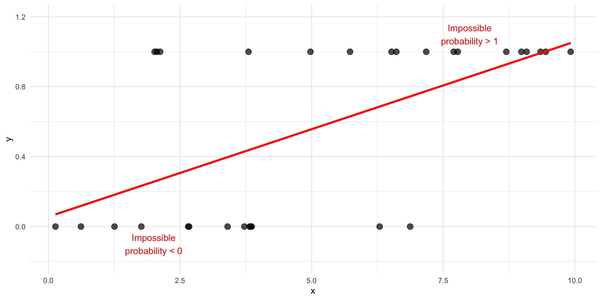
- Responses are only 0 or 1
- We want to estimate a probability
- Probabilities must be between 0 and 1
- Linear regression can predict values less than 0 or greater than 1
Logistic Regression
- Given a data set that has a (binary) qualitative predictor, the two categories can be thought of as complementary states for a probability formulation.
- Then, logistic regression can model the probability of one state of interest.
- For example, consider the book’s data set on credit default. We are interested in modelling the probability of default for a given creditor. Then, for any combination of predictors, we can make a prediction of default.
- How do we do this?
The Logistic Model
- We write \(p(X) = \Pr(Y = 1 | X)\), and will use it to model the relationship between \(p(X)\) and \(X\).
- We need a function that gives values between \(0\) and \(1\) (to be valid probabilities), regardless of the infinite possible values for \(X\).
- Many functions can do this, but for technical reasons, we will use the logistic function:
\[ p(X) = \frac{e^{\beta_0 + \beta_1 X}}{1 + e^{\beta_0 + \beta_1 X}}. \]
The Logistic Curve
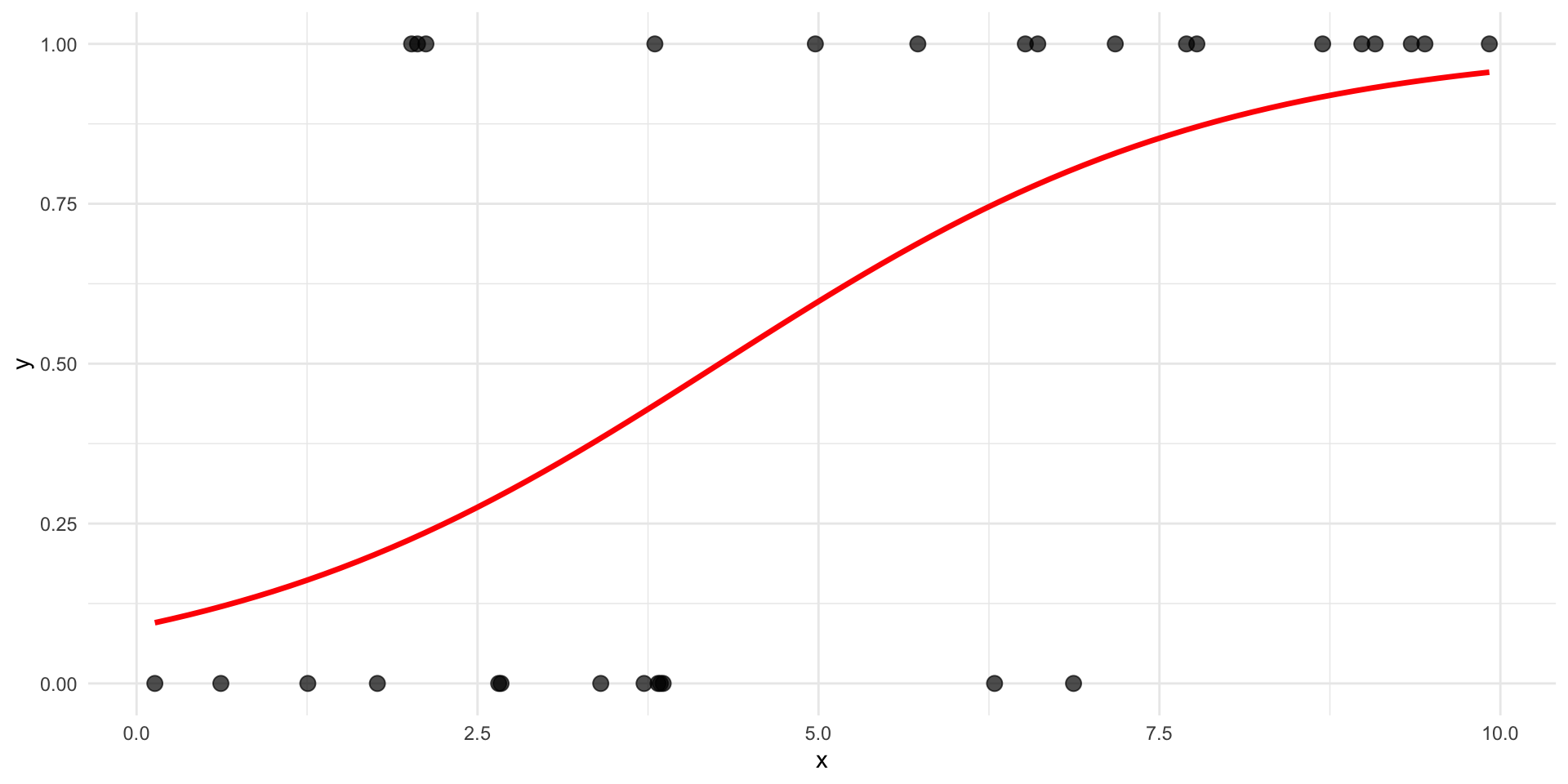
- Predictions are always between 0 and 1
- Produces probabilities
- Allows non-linear probability curves
Tip
No matter how large or small \(x\) becomes, the predicted probability remains valid.
Technical Note
- Logistic regression models are not fit using least squares like regression.
- Instead, they use a technique called maximum likelihood, that does some minimax operations to find the likelihood parameters that maximize the fit to data.
- This means that when we run the models in R, the outputs aren’t going to look exactly the same as for regression. Similar, but not the same!
Some Alternative Representations
If we manipulate the primary relationship from above, we can find
\[ \frac{p(X)}{1 - p(X)} = e^{\beta_0 + \beta_1 X}. \] The left hand side of this expression is called the odds (or odds ratio), and is between 0 and infinity.
Another Representation
- Take the logarithm of both sides of the previous: \[ \log\left( \frac{p(X)}{1 - p(X)} \right) = \beta_0 + \beta_1 X. \]
- The left hand side here is called the logit (or log odds), and this model is linear in \(X\).
- This has a somewhat nice interpretation: if we increase \(X\) by one unit, this changes the log odds by \(\beta_1\). This is equivalent to multiplying the odds by \(e^{\beta_1}\).
- However: \(p(X)\) is not related linearly, so this doesn’t give a nice relationship between \(X\) and \(p(X)\) - it’s not possible!
Maximum Likelihood Estimation
- Although we could use (non-linear) least squares to fit the model, the more general method of maximum likelihood is preferred, since it has better statistical properties.
- The basic intuition behind using maximum likelihood to fit a logistic regression model is as follows:
- We seek estimates for \(\beta_0\) and \(\beta_1\) such that the predicted probability \(\hat{p}(x_i)\) for each obsevation, using the formula given, corresponds as closely as possible to the observation’s observed response status.
- In other words: find the \(\hat{\beta_0}\) and \(\hat{\beta_1}\) such that plugging these estimates into the model for \(p(X)\) gives predictions that are close to the correct states for the response variable observed.
An Example: Credit Card Default
Let’s use the default dataset which is mentioned in the textbook, along with a predictor balance, which refers to credit card balances.
An Example: Credit Card Default
- It’s possible that we could run into issues because
defaultis coded as a factor instead of a logical (glm()uses the second level of the factor by default). - I’ll recode to be safe:
Rows: 10,000
Columns: 4
$ default <lgl> FALSE, FALSE, FALSE, FALSE, FALSE, FALSE, FALSE, FALSE, FALSE,…
$ student <lgl> FALSE, TRUE, FALSE, FALSE, FALSE, TRUE, FALSE, TRUE, FALSE, FA…
$ balance <dbl> 729.5265, 817.1804, 1073.5492, 529.2506, 785.6559, 919.5885, 8…
$ income  <dbl> 44361.625, 12106.135, 31767.139, 35704.494, 38463.496, 7491.55…
The Model: Credit Card Default
  default student   balance    income
1   FALSE   FALSE  729.5265 44361.625
2   FALSE    TRUE  817.1804 12106.135
3   FALSE   FALSE 1073.5492 31767.139
4   FALSE   FALSE  529.2506 35704.494
5   FALSE   FALSE  785.6559 38463.496
6   FALSE    TRUE  919.5885  7491.559
So we have default status (whether or not they defaulted on their debt), student status, credit card balance, and income. We will start with a simple model, \[\text{default} \sim \beta_0 + \beta_1 \text{balance}\]
Default Example (ctd.)
Call:
glm(formula = default ~ balance, family = binomial, data = Default)

Coefficients:
              Estimate Std. Error z value Pr(>|z|)
(Intercept) -1.065e+01  3.612e-01  -29.49   <2e-16 ***
balance      5.499e-03  2.204e-04   24.95   <2e-16 ***
---
Signif. codes:  0 '***' 0.001 '**' 0.01 '*' 0.05 '.' 0.1 ' ' 1

(Dispersion parameter for binomial family taken to be 1)

    Null deviance: 2920.6  on 9999  degrees of freedom
Residual deviance: 1596.5  on 9998  degrees of freedom
AIC: 1600.5

Number of Fisher Scoring iterations: 8
Interpreting the Coefficients
                 Estimate   Std. Error   z value      Pr(>|z|)
(Intercept) -10.651330614 0.3611573721 -29.49221 3.623124e-191
balance 0.005498917 0.0002203702 24.95309 1.976602e-137- The setup is basically the same as for multiple linear regression, except that the interpretation is different, as discussed earlier.
- We see that \(\hat{\beta_1} = 0.0055\), which indicates that an increase in balance is associated with an increase in the probability of default.
- To be precise, a thousand-unit increase in balance (so an additional $1,000 credit card balance) is associated with an increase in the log odds of default of 5.5 units.
Making Predictions
- Once we have coefficients, we can compute probabilities of default for any given credit card balance.
- If we do this manually, it requires substituting into the \(p(X)\) formula from earlier, e.g., for a balance of $1,000: \[ \hat{p}(1000) = \frac{e^{-10.6513 + 0.0055 \times 1000}}{1 + e^{-10.6513 + 0.0055 \times 1000}} = 0.00576. \] Thus, the probability of default for an individual with a credit card balance of $1,000 is 0.6%: not very high!
Making Predictions (Continued)
By contrast, someone with a balance of $3,000 has: \[ \hat{p}(3000) = \frac{e^{-10.6513 + 0.0055 \times 3000}}{1 + e^{-10.6513 + 0.0055 \times 3000}} = 0.997, \] or an almost certain probability of default, given this data set as training, and using no other predictive factors.
Dummy Predictor Variables
- We can also use qualitative predictor variables if we like.
- For example, we can use the variable
studentto predict instead, where student is a True/False Boolean variable.
Dummy Predictor Variables
Call:
glm(formula = default ~ student, family = binomial, data = Default)

Coefficients:
            Estimate Std. Error z value Pr(>|z|)
(Intercept) -3.50413    0.07071  -49.55  < 2e-16 ***
studentTRUE  0.40489    0.11502    3.52 0.000431 ***
---
Signif. codes:  0 '***' 0.001 '**' 0.01 '*' 0.05 '.' 0.1 ' ' 1

(Dispersion parameter for binomial family taken to be 1)

    Null deviance: 2920.6  on 9999  degrees of freedom
Residual deviance: 2908.7  on 9998  degrees of freedom
AIC: 2912.7

Number of Fisher Scoring iterations: 6
Interpretation
Same as before, except with a qualitative predictor: \[ \begin{split} \hat{\Pr}(\text{default = TRUE} \,|\, \text{student = TRUE}) &= \frac{e^{-3.5041 + 0.4049 \times 1}}{1 + e^{-3.5041 + 0.4049 \times 1}}\\ &= 0.0431 \end{split} \] versus…
Interpretation
\[ \begin{split} \hat{\Pr}(\text{default = TRUE}\, | \,\text{student = FALSE}) &= \frac{e^{-3.5041 + 0.4049 \times 0}}{1 + e^{-3.5041 + 0.4049 \times 0}} \\ &= 0.0292.\end{split} \]
- So, students tend to have higher default probabilities than non-students.
- This perhaps is not surprising given that students are under unique stressors, and have additional expenses and limited income as compared to non-students (who presumably are working adults).
Multiple Logistic Regression
Multiple Regression, but Logistic
We can generalize logistic regression to multiple logistic regression in exactly the same way we did for multiple regression, resulting in: \[ p(X) = \frac{e^{\beta_0 + \beta_1 X_1 + \cdots + \beta_p X_p}}{1 + e^{\beta_0 + \beta_1 X_1 + \cdots + \beta_p X_p}}. \]
Example, again using Default
Use all three available variables to predict default:
Example, again using Default
Call:
glm(formula = default ~ balance + income + student, family = binomial,
    data = Default)

Coefficients:
              Estimate Std. Error z value Pr(>|z|)
(Intercept) -1.087e+01  4.923e-01 -22.080  < 2e-16 ***
balance      5.737e-03  2.319e-04  24.738  < 2e-16 ***
income       3.033e-06  8.203e-06   0.370  0.71152
studentTRUE -6.468e-01  2.363e-01  -2.738  0.00619 **
---
Signif. codes:  0 '***' 0.001 '**' 0.01 '*' 0.05 '.' 0.1 ' ' 1

(Dispersion parameter for binomial family taken to be 1)

    Null deviance: 2920.6  on 9999  degrees of freedom
Residual deviance: 1571.5  on 9996  degrees of freedom
AIC: 1579.5

Number of Fisher Scoring iterations: 8
Surprising Interpretation
- Notice that we have very small \(p\)-values for both balance and student.
- However, the coefficient of student is negative here: indicating that students are less likely to default than non-students. Isn’t that the exact opposite of what we saw before?
- The negative coefficient for student in the multiple logistic regression indicates that for a fixed value of balance and income, a student is less likely to default than a non-student…
Surprising Interpretation
- However, the overall student default rate is higher than the non-student default rate.
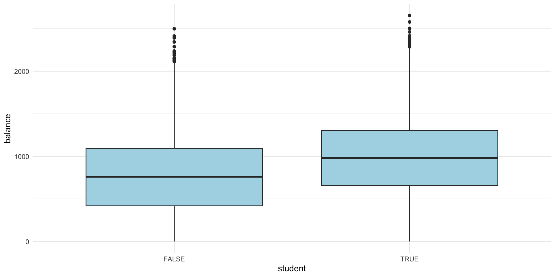
- Consequently, there is a positive coefficient for student in the single variable model. So why?
Surprising Interpretation
- The variables student and balance are correlated.
- Students generally carry higher credit card balances, and higher balances are linked to greater default risk.
- This means that although a student with a given balance is less likely to default than a non-student with the same balance.
- The fact that students as a group tend to have larger balances leads to higher overall default rates among students.
- This distinction is important for credit card companies when deciding to whom to offer credit.
Surprising Interpretation
- This simple example illustrates the dangers and subtleties associated with performing regressions involving only a single predictor when other predictors may also be relevant.
- As in the linear regression setting, the results obtained using one predictor may be quite different from those obtained using multiple predictors, especially when there is correlation among the predictors.
- In general, the phenomenon seen here is known as confounding.
Predicting
We can use the same predict methods as before to predict a specific result.
         1
0.05788194 1
-2.789725 [1] -2.789726This means an estimated probability of default of 0.0578819, which corresponds to log odds of -2.7897251
Confusion Matrices
The so-called confusion matrix compares logistic regression predictions to the true statuses.
         logclass
trueclass FALSE TRUE
    FALSE  9627   40
    TRUE    228  105
Diagonal elements are correct predictions; off-diagonal elements are incorrect classifications. Thus, the error rate is (40+228)/10000*100% = 2.68%.
Some Notes on Error Rate
- training error rates will usually be lower than test error rates, which are the real quantity of interest. In other words, we might expect this classifier to perform worse if we use it to predict whether or not a new set of individuals will default.
- Since only 3.33% of the individuals in the training sample defaulted, a simple but useless classifier that always predicts that an individual will not default will result in an error rate of 3.33 %. In other words, the trivial null classifier will achieve an error rate that is only a bit higher than the logistic regression training set error rate.
A Further Note
- Of the 333 individuals who truly defaulted, 228 (or 68.5%) were missed by logistic regression.
- So while the overall error rate is low, the error rate among individuals who defaulted is very high.
- From the perspective of a credit card company that is trying to identify high-risk individuals, an error rate of 228/333 = 68.5 % among individuals who default should be unacceptable!
Some Definitions
- Class-specific performance is also important in medicine and biology, where the terms sensitivity and specificity characterize the performance of sensitivity a classifier or screening test.
- Sensitivity is a test’s ability to correctly identify people who have a condition (the true positive rate).
- Specificity is a test’s ability to correctly identify people who do not have a condition (the true negative rate).
- In our case the sensitivity is the percentage of true defaulters that are identified; it equals 31.5%. The specificity is the percentage of non-defaulters that are correctly identified; it equals 9627/9667 = 99.6%.
confusionMatrix()
Confusion Matrix and Statistics

          Reference
Prediction FALSE TRUE
     FALSE  9627  228
     TRUE     40  105

               Accuracy : 0.9732
                 95% CI : (0.9698, 0.9763)
    No Information Rate : 0.9667
    P-Value [Acc > NIR] : 0.0001044

                  Kappa : 0.4278

 Mcnemar's Test P-Value : < 2.2e-16

            Sensitivity : 0.3153
            Specificity : 0.9959
         Pos Pred Value : 0.7241
         Neg Pred Value : 0.9769
             Prevalence : 0.0333
         Detection Rate : 0.0105
   Detection Prevalence : 0.0145
      Balanced Accuracy : 0.6556

       'Positive' Class : TRUE
Discriminant Analysis
Discriminant Analysis
- Logistic regression involves directly modelling \(\Pr(Y = k|X = x)\) using the logistic function.
- We now consider an alternative and less direct approach to estimating these probabilities.
- In this new approach, we model the distribution of the predictors \(X\) separately in each of the response classes (i.e., for each value of Y ).
- We then use Bayes’ Theorem to flip these around into estimates for \(\Pr(Y = k|X = x)\).
- When the distribution of \(X\) within each class is assumed to be normal, it turns out that the model is very similar in form to logistic regression.
Why Do We Need This?
- When there is substantial separation between the two classes, the parameter estimates for the logistic regression model are surprisingly unstable.
- The methods that we consider in this section do not suffer from this problem.
- If the distribution of the predictors \(X\) is approximately normal in each of the classes and the sample size is small, then the approaches in this section may be more accurate than logistic regression.
Some Background
- Suppose that we wish to classify an observation into one of \(K\) classes, where \(K \geq 2\).
- In other words, the qualitative response variable \(Y\) can take on \(K\) possible distinct and unordered values.
- Let \(\pi_k\) represent the overall or prior probability that a randomly chosen observation comes from the prior \(k^\text{th}\) class.
Some Background
- Let \(f_k(X) = \Pr(X|Y = k)\) denote the density function of \(X\) for an observation that comes from the \(k^\text{th}\) class.
- In other words, \(f_k(x)\) is relatively large if there is a high probability that an observation in the \(k^\text{th}\) class has \(X \approx x\), and \(f_k(x)\) is small if it is very unlikely that an observation in the \(k^\text{th}\) class has \(X \approx x\).
- Then Bayes’ theorem states that \[ \Pr(Y = k|X=x) = \frac{\pi_k f_k(x)}{\sum_{j=1}^{K} \pi_j f_j(x)}. \]
Simpler Notation
- We will use the same abbreviated notation as earlier: \[ p_k(x) = \Pr(Y = k|X=x), \] the posterior probability that an observation \(X=x\) belongs to the \(k^\text{th}\) class.
- Or, in other words, the probability that an observation belongs to the \(k^\text{th}\) class, given the predictor value for that observation.
- We will need to estimate \(\pi_k\) and \(f_k(x)\). There are a number of ways we can try to do this.
Linear Discriminant Analysis for p = 1
- Assume \(p=1\), that is, only one predictor (like simple linear regression or simple logistic regression).
- We want an estimate of \(f_k(x)\) to plug in.
- To do this, we assume \(f_k(x)\) is Gaussian, and that the variances are the same for each of the \(K\) classes (denote this by \(\sigma^2\)).
- There’s a mathematical derivation in the text, but our method will use Linear Discriminant Analysis (LDA) to approximate this theory, by computing estimates of \(\mu_1\) through \(\mu_K\), \(\pi_1\) through \(\pi_k\), and \(\sigma^2\), and then plug them in to estimate which class each observation should be assigned to.
An Example - Default, but with LDA
Use the Default data set again, but apply LDA to it.
Call:
lda(default ~ balance + student, data = Default)

Prior probabilities of groups:
 FALSE   TRUE
0.9667 0.0333

Group means:
        balance studentTRUE
FALSE  803.9438   0.2914037
TRUE  1747.8217   0.3813814

Coefficients of linear discriminants:
                     LD1
balance      0.002244397
studentTRUE -0.249059498
An Example - Default, but with LDA
An Example - Default, with LDA
The LDA output indicates that \(\hat{\pi}_1 = 0.9667\) and \(\hat{\pi}_2 = 0.0333.\) In other words, 96.7% of the training observations correspond to non-default and 3.33% to default (this exactly matches).
It also provides the group means; these are the average of each predictor within each class, and are used by LDA as estimates of \(\mu_k\).
An Example - Default, with LDA
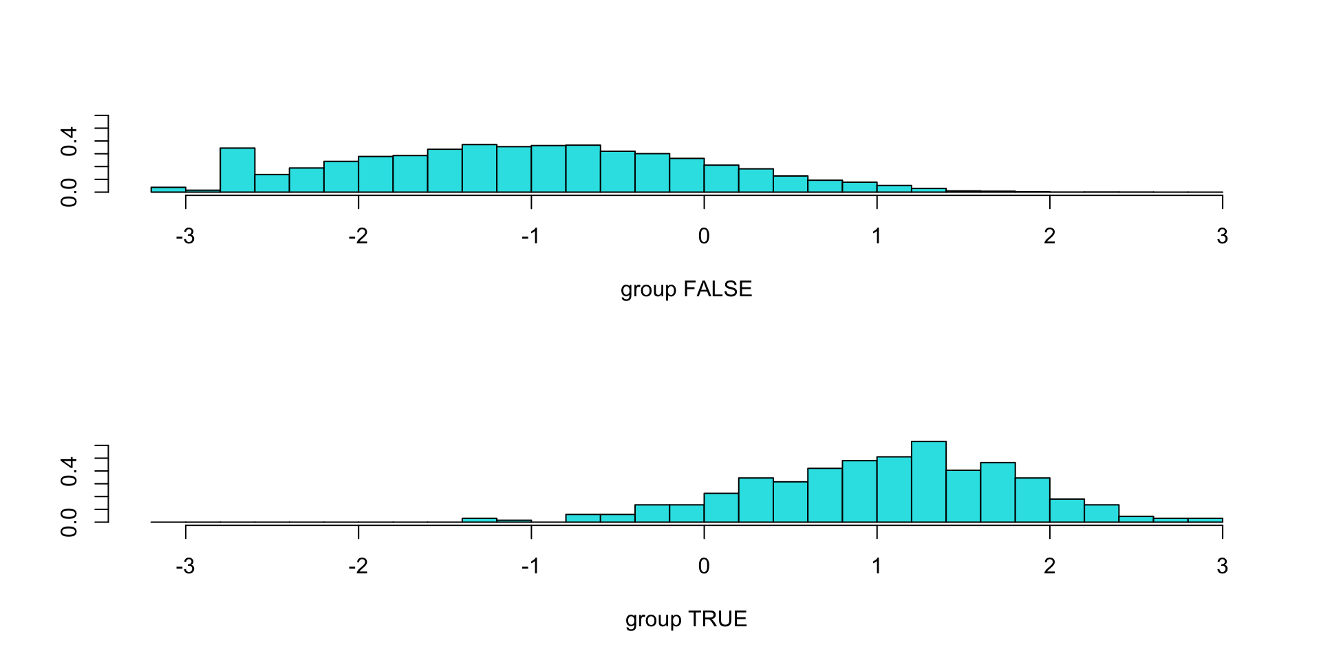
- The coefficients of linear discriminant output provides the linear combination of balance and student-status that are used to form the LDA decision rule.
- If \(0.00224\times\text{balance}-0.2491\times \text{student}\) is large, then the LDA classifier will predict a default, and if it is small, then a non-default.
- Remember that student is a binary variable with 0 meaning “No”/ FALSE and 1 meaning “Yes”/ TRUE.
An Example - Default, with LDA
pred_lda <- predict(mod4)
data.frame(Pred_Class = pred_lda$class, LDA_Score = pred_lda$x) |>
  ggplot(aes(x = Pred_Class, y = LD1, fill = Pred_Class)) + geom_boxplot() +
  theme_minimal() + theme(legend.position = "none")+
  labs(x = "Predicted Class", y = "LDA Score") +
  geom_hline(yintercept = 2.586084, colour = "red", linetype = "dashed")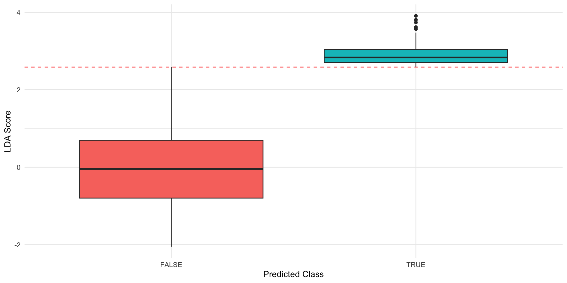
Pulling out the Predictions
Pulling out the Predictions
      FALSE        TRUE
1 0.9968680 0.003131975
2 0.9971925 0.002807531
3 0.9843970 0.015603046
4 0.9987769 0.001223133
5 0.9959254 0.004074582
6 0.9954627 0.004537289
The TRUE category here corresponds to our \(p_k(x)\).
Compare the Predictions
- Recall that
mod3was our logistic regression classifier from earlier. - By default, the classifier applies a 50% threshold - that is, a prediction of less than 0.50 is classified as FALSE, while a prediction above 0.50 is classified as TRUE.
- Let’s compare the classifications from the LDA and our earlier logistic model.
Compare the Predictions
Confusion Matrix and Statistics

          Reference
Prediction FALSE TRUE
     FALSE  9627  228
     TRUE     40  105

               Accuracy : 0.9732
                 95% CI : (0.9698, 0.9763)
    No Information Rate : 0.9667
    P-Value [Acc > NIR] : 0.0001044

                  Kappa : 0.4278

 Mcnemar's Test P-Value : < 2.2e-16

            Sensitivity : 0.3153
            Specificity : 0.9959
         Pos Pred Value : 0.7241
         Neg Pred Value : 0.9769
             Prevalence : 0.0333
         Detection Rate : 0.0105
   Detection Prevalence : 0.0145
      Balanced Accuracy : 0.6556

       'Positive' Class : TRUE
Confusion Matrix and Statistics

          Reference
Prediction FALSE TRUE
     FALSE  9644  252
     TRUE     23   81

               Accuracy : 0.9725
                 95% CI : (0.9691, 0.9756)
    No Information Rate : 0.9667
    P-Value [Acc > NIR] : 0.0004973

                  Kappa : 0.3606

 Mcnemar's Test P-Value : < 2.2e-16

            Sensitivity : 0.2432
            Specificity : 0.9976
         Pos Pred Value : 0.7788
         Neg Pred Value : 0.9745
             Prevalence : 0.0333
         Detection Rate : 0.0081
   Detection Prevalence : 0.0104
      Balanced Accuracy : 0.6204

       'Positive' Class : TRUE
Setting Thresholds
- By default, the LDA classifier classifies based on a which class has the highest posterior probability.
- This is a 50% threshold in our two-class case.
- By default, logistic regression predicts a credit default when the predicted probability is above 50%. This is configurable.
- In the case of the Default data set, maybe we want to label any custom with a posterior probability of credit default above 20% to the default class. That is, \[ \Pr(\text{default = TRUE} | X=x) > 0.2. \]
Changing the Threshold
We can do this manually:
Naive Bayes
A Final Classifier
- So far we’ve discussed logistic regression and LDA. There is a third method we will discuss, called Naive Bayes.
- In the earlier derivations, we needed estimates of \(\pi_1, \cdots, \pi_K\), and also \(f_1(x), \cdots, f_K(x)\).
- The LDA algorithms estimated the \(\pi_i\) quantities by using the proportion of training observations belonging to the \(k^\text{th}\) class.
- Then, estimating the functions \(f_i(x)\) was more complicated, and we left it to the code.
- In LDA, we made a very strong assumption: that \(f_k\) were density functions for Gaussian random variables.
- Our final method uses quite a different approach.
Naive Bayes
Instead of assuming that the functions \(f_k(x)\) belong to a particular family of distributions, we instead make a single assumption:
Within the \(k\)th class, the \(p\) predictors are independent
- This is very powerful because it allows us to simplify the joint distribution !
- By assuming that the \(p\) covariates are independent within each class, we completely eliminate the need to worry about the association between the \(p\) predictors, because we have simply assumed that there is none!
Do We Really Believe This?
- In most settings, we do not.
- But even though this modelling assumption is made for convenience, it often leads to pretty decent results, especially in settings where \(n\) is not large enough relative to \(p\) for us to effectively estimate the joint distribution of the predictors within each class.
- Essentially, the naive Bayes assumption introduces some bias, but reduces variance, leading to a classifier that works quite well in practice as a result of the bias-variance trade-off.
Applying Naive Bayes
$balance
       balance
Y            [,1]     [,2]
  FALSE  803.9438 456.4762
  TRUE  1747.8217 341.2668

$student
       student
Y           FALSE      TRUE
  FALSE 0.7085963 0.2914037
TRUE 0.6186186 0.3813814 nbclass
trueclass FALSE TRUE
FALSE 9621 46
TRUE 244 89Changing the Threshold
Again, we can change the threshold if we like:
Summary
- Classification is a highly powerful topic, which is very useful for modelling the real world, where we often want to make these kinds of judgement calls - Yes/No, or multinomial.
- We have discussed three classes of solvers today: logistic regression; linear discriminant analysis; and naive Bayes.
- All have strengths and weaknesses, and all are reasonably simple if you have access to R.
- We will explore a full worked example of an interesting data set shortly.
Comparing Classification Methods
| Method | Main Idea | Key Assumption(s) | Advantages | Disadvantages |
|---|---|---|---|---|
| Logistic Regression | Models the probability of belonging to a class directly | Linear relationship between predictors and log-odds | Easy to interpret; provides probabilities; few assumptions | Can struggle with strong class separation |
| LDA | Models the distribution of predictors within each class and applies Bayes’ theorem | Predictors are normally distributed with equal variances across classes | Can perform well with small samples; often very stable | Requires stronger distributional assumptions |
| Naive Bayes | Models predictor distributions assuming conditional independence | Predictors are independent within each class | Fast; works surprisingly well in practice; handles many predictors | Independence assumption is often unrealistic |
Next Topic
Our first major topic will be on validating models that we’ve fit, using cross-validation and the bootstrap, and starting a discussion of proper, modern methods for choosing variables in a model!
Readings
The material of this week is Chapter 4 of ISLR, sections 4.1-4.6.
Next week, we will continue into Chapters 5 and 6, and discuss model validation and variable selection. Readings are Chapters 5.1, 5.2, and 6.1-6.3.